Results

We performed several tests to evaluate the applicability of bcc grids. First, we compared our gradient reconstruction schemes to the commonly used central differences on Cartesian grids. Then, we modified an existing splatter to operate on bcc grids. Finally, as sampling on bcc grids results in a compression of the data, we also compared it to existing compression techniques for volumetric data.

Gradient estimation

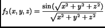
In order to evaluate the quality of the gradient approximation we used three different analytical functions for comparison purposes:

• spherical with linear falloff:

  $$f_1(x, y, z) = \sqrt{x^2+y^2+z^2}$$ (25)

  
  

• Sinc function:

  $$f_2(x, y, z) = \frac{\sin(\sqrt{x^2+y^2+z^2})}{\sqrt{x^2+y^2+z^2}}$$ (26)

  
  

• simplified Marschner-Lobb:

  $$f_3(x, y, z) = \sin(x^2+y^2+z^2)$$ (27)

  
  

We computed the actual function values at the positions defined by the bcc grid so that no errors were introduced during the sampling process. We then applied our two gradient reconstruction schemes and computed the difference of the normals with the analytically computed normals at the sampling grid. We recorded two errors - the error in the magnitude of the normal as well as the angular error in the normal. We then looked at these errors in one slice at a time. Since in our indexing scheme an xy-slice (z is constant) is easy to extract we chose xy slices. Furthermore, we were interested in how well these errors compare to errors introduced by central differences and linear filtering on regular rectilinear grids. Hence we computed the normals as if the original data set was given on a rectangular grid using central differences and linear interpolation.

The results of our experiment can be seen in Fig 7 (a) - (c). The first row shows the relative error in magnitude and the second row shows the angular error. Column one depicts the error of our first gradient reconstruction method (Eq. 22) that is based on central differences at the grid point itself. Column 2 corresponds to method two (Eq. 23), which is the average of all central differences at the of the cube edges surrounding the sampling point. In the last column we computed the linearly interpolated central differences, assuming the data set was given on a regular grid with corresponding dimensions.

Fig 7(a) shows the error images for function $f_1$. In this image an angular error of 15 degrees and an amplitude error of 30% corresponds to white (255). Fig. 7(b) shows the error images for function $f_2$. Here an angular error of 30 degrees and an amplitude error of 60% corresponds to white (255). Finally the results for function $f_3$ are displayed in Fig. 7(c). Here 5 degrees for the angular error and 10% for the amplitude error correspond to white (255).

Figure 7: Difference images of analytically calculated gradients to our gradient estimation schemes (see Sec. 3.3), first two columns, and central differences with linear interpolation, third column, for (a) sphere, (b) Sinc, and (c) simplified Marschner-Lobb function. The top rows show the error in magnitude whereas the bottom rows show the angular error.(a) error in magnitude by 30% and an angular error of 15 degrees corresponds to white, (b) amplitude error of 60% and an angular error of 30 degrees corresponds to white, (c) amplitude error of 10% and an angular error of 5 degrees corresponds to white.

(a)
    

(b)
    

(c)
    

From these images we conclude that both our difference methods are quite comparable with central differencing and linear interpolation on regular grids. Hence one need not to worry about quality loss by using bcc grids for volume rendering applications. Furthermore since there are no large differences between the two introduced methods in Section 3.3, we don't find the expensive operations of method 2 justified.

Splatting

We rendered several different data sets using both a usual Cartesian grid and a bcc grid. All images were generated using the same transfer function and viewing parameters.

Fig. 8 shows images of the Marschner-Lobb data set sampled on a $40\times 40\times 40$ Cartesian grid (as described by Marschner and Lobb [11]) on the left respectively a $28 \times 28\times 56$ bcc grid on the right. This data set is quite demanding for a straightforward splatter and there are some visible differences in the results. The image generated from the bcc grid is rather blurred whereas the image from the Cartesian grid exhibits strong artifacts, especially in diagonal directions.

Figure 8: Marschner-Lobb data set rendered by splatting with a Cartesian grid on the left and a bcc grid on the right.

The data sets that we used for rendering the images in Color Plate 1 were produced using a high-quality interpolation filter. We used the $C^3$-4EF filter as designed by Möller et al. [13]. In Color Plate 1 we show results of rendering the ``neghip'' data set as well as the High Potential Iron Protein data set by Louis Noodleman and David Case, of Scripps Clinic, La Jolla, California, as well as the fuel injection data set. Again, a regular Cartesian grid was used on the left and a bcc grid on the right. There are some visible differences in the images. Since we classify different values that represent two different grid positions one cannot expect identical pictures. Hence we see some differences resulting from the problem of pre-classification [20].

Color Plate 1: Images generated via splatting on a Cartesian grid on the left respectively a body-centered cubic grid on the right. The body-centered cubic grids require approximately 30% less samples. Small differences are visible, that likely are caused by pre-classification.

Cartesian grid	body-centered cubic grid

We also did some timings which are reported in Table 1. It is interesting to note that the speedup for some data sets were bigger than expected. This could have been caused by the decreased memory caching necessary. For a very small data set (lobster) we saw expected speedups near 30%.

Table 1: Timings for several different datasets are reported in seconds per frame.

Data set	rectilinear	bcc grid	speedup
uncbrain	1.51	0.8	47%
hipip	0.103	0.059	43%
lobster	0.056	0.043	23%

Compression

Our results indicate that the resampled data have the potential to lead to better compression. We were able to show that our compression ratios for practical data sets are better than what was achieved using the gzip utility. Also, our overall compression ratios were better then previously reported [5]. Table 2 shows compression ratios of various volume data sets. Note that the last two columns give percentages as compared to the original data size indicating the overall compression ratio, which is what we are interested in. However, the compression of synthetic data sets is a rather surprising result and needs to be further investigated.

Table 2: Compression ratios of several volume data sets. The last two columns give the percentage as compared to the original data size.

	original	bcc grid	original (gzipped)	bcc (gzipped)	% original	% bcc
uncbrain	9502732	6716017	4547141	2948524	47.8	31.0
nerve	19922955	14021720	8819382	5744443	44.3	28.8
ultrasound	6291467	4422747	4347958	3140634	69.1	49.9
tetrahedron	92410	64024	7028	14456	7.6	15.6
Marschner-Lobb	64001	43913	22823	34861	35.7	54.5