User Guide |
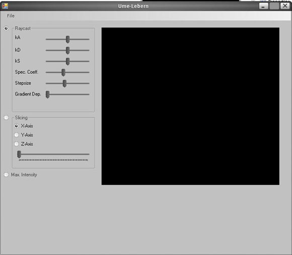
Contents: After starting Ume-Lebern, you will see a screen like this:
You can load a data set using the file dialog "File -> Open". Some data sets can be found at the VisLab homepage. To render and save the image you see in the main window, click "File -> Render HighRes...". Enter width and height, choose a file name and klick enter. At the left, you can use the radio buttons to switch through the Visualisation techniques. Refer to the next chapters for a more detailed explanation of them. The main window displays the object using the selected rendering method. Click your mouse to rotate it, or right click and move your mouse back and forth to zoom in and out. Click your middle mouse button to rotate the light source around the object. While rotating the light source or the object, the image is rendered in a lower resolution to show the changes at interactive framerates. After you "drop" the mouse, the image is refined. At the bottom of the screen you can see the density histogram of the loaded object. Less dense layers are located at the left, more dense layers at the right. The amplitude shows the logarithm of the quantity this density appears with. You can now interactively add points by clicking into the histogram and move them by drag and drop. This creates a function approximated by discrete points and interpolated linearly between them, that is used to apply a certain opacity to each density. The higher the function at a certain density, the more opacity is used when rendering these layers. Additionally, you can apply a color to each point by double-clicking it. This will cause the renderer to use this color to display this density. Again, colors are interpolated linearly between the points.
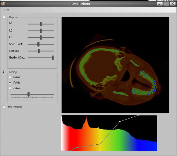
Load a data set and select "Slicing". You can now choose one of the main axes. Use the Slider to change the value to slice through the data set. A slice will be drawn at the point the slider position corresponds to at the selected axis.
Slices are drawn as quads in 3D Space, so they can be rotated and zoomed as well. Load a data set and select "Raytracing" to render the data by depth compositing using the algorithm proposed by Levoy [^]. Shading is done by a standard phong illumination model, using the gradient at a point as normal. Use the transfer function as described above to adjust color and opacity for certain density levels. You will soon see that you can extract multiple semi-transparent layers to get an image like this:
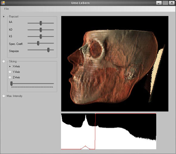
By changing the stepsize you can boost the quality of the image. But since Shader 3.0 cards stop iterating a loop after some 250 iterations, setting the stepsize slider to the right (which, not very intuitivly corresponds to a very small stepsize) may cause the farther regions of the object to disappear. Advanced gradient dependent opacity computation As an extended feature, we have implemented a render mode that takes the length of the gradient into account when computing the opacity. This has the effect that edges are rendered with a higher opacity and are therefore more visible and opaque. You can change the gradient dependency by changing the slider "Gradient Dep" when rendering in raytrace mode. This picture was composed from a rendering with low (upper half) and high gradient dependent dependent opacity computation:
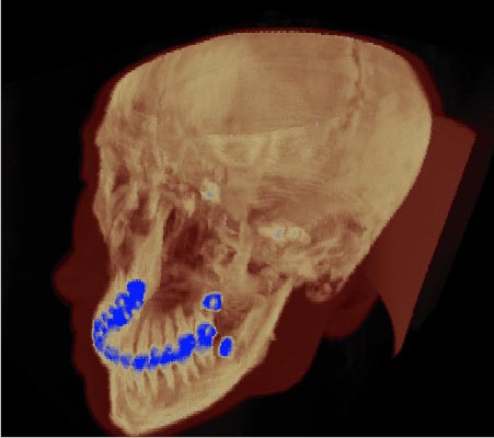
Select the last radio button for MIP (maximum intensity projection) rendering. Unlike depth compositing, MIP just shows the color of the point with the maximal density along a ray path. Colors are again taken from the transfer function.
As you can see here, the person scanned did not get his wisdom teeth - at least not on the left ;-)
|