User interface Guide
Contents
- Interface Components
- Using Slices
- Editing the Transfer Function with Slices
- Using Raycasting
Interface Components
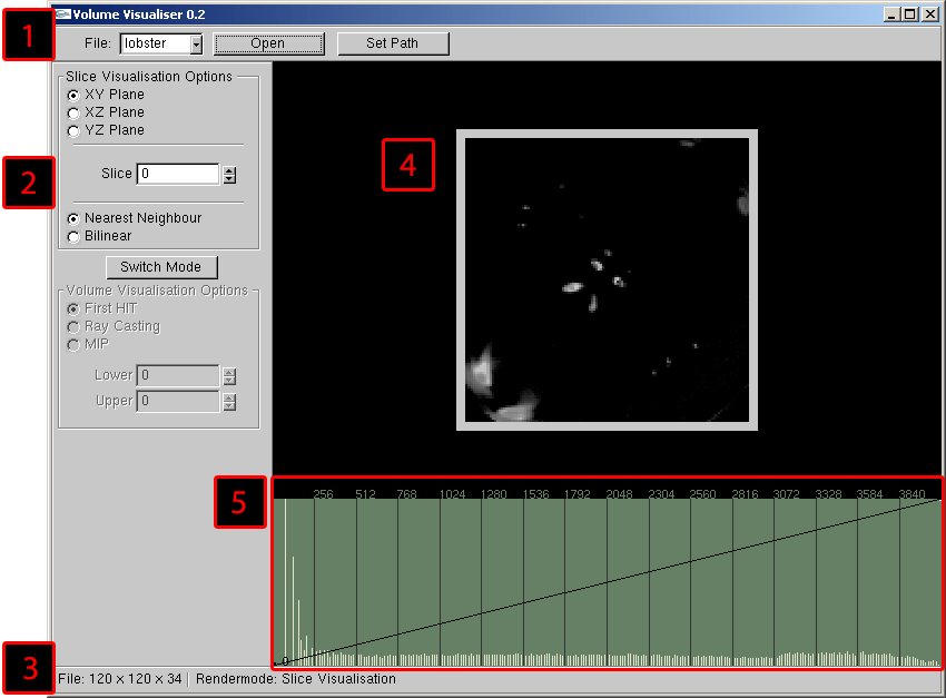
The interface is desined to be as simple and intuitive as possible. It is made of three basic components: the (1)Menubar, the (2)Option Panel, the (3)Statebar, the (4)Rendering Area and the (5)Histogram.. Some components are only visible at certain states of the program and will be described later (e.g. the Histogram).
Standard UI Components
(1)Menubar, (2)Option Panel, (3)Statebar, (4)Rendering Area, (5)Histogram.
The menu bar provides the functionality to load serveral *.dat files. If the program does not find any valid data file in the /data subdirectory, the user is only able to set a path. The path determines where the program should search for files and is given relative or absolute to the execution path. If the path does provide any valid file or can not be found, the ann error message will appear.
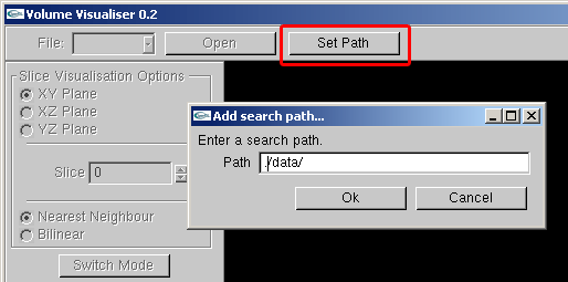
Set Path Dialog. If the path is not correct, an error message will be shown.
Once the path is set (correct), valid *.dat files are extracted and their names are stored in a drop down list. The user can now select one of these names and press open. The program will then load the file - wich is shown in the statebar. Once the loading has finished, the program enters the slicing mode.
The option panel lets the user select between the two render modes: slicing mode and raycasting.. Therefor he needs to press the Switch Mode Button.
Loading and preprocessing volume data takes usually more or less time. Note that the Statebar is alway showing the state of the program. (Hey this sentence could be from an MS help file:-)
How to use Slicing
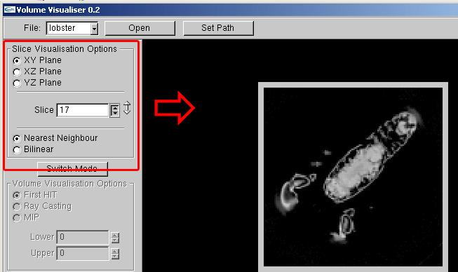
Once a dataset had been loaded the user can step through the data in slicing mode. In this mode, the statebar shows the message Rendermode: Slice Visualisation and the upper part of the option panel is activated. The user can select the following options
- Axis Aligned Viewing Direction
- The slice number.
- The texture interpolation method
Each option takes effect immediatly in the rendering area. I.e when enter a slice number, the slice should be visible. It is also possible to click with the mouse on the spinner and drag, to select a slice.
Active Options in Slicing mode.
To change the image quality, the user can change between nearest neighbor and Bilinear Interpolation. This will change the OpenGL filterring.
Editing the Transfer Function with Slices
Beside setting options with the options panel, the user can change the appearance of the slice using the transferfunction editor. The use is straight forward by adding control points to a certain density in the histogram.
After loading a dataset, the histogram appears at the bottom. It contains the occurencies of each density in the dataset (Note: The density of 0 is not counted). The vertical bars should give the user the abbility to guess, wich density occurs how often.
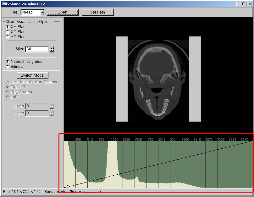
The Histogram in initial state. The numbers showing intervalls of densities.
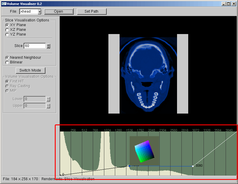
To specify a color for a density in the resulting image, the user defines so called control points. Therefore the user needs to click with the left mouse button on the histogram. Initially this adds a control point with white color. It is also possible to grab and drag an defined controlpoint. Since the resulting color for each density in the image is then interpolated linearly between the nearest two control points, adding and changing the position of a point takes effect immediatly.
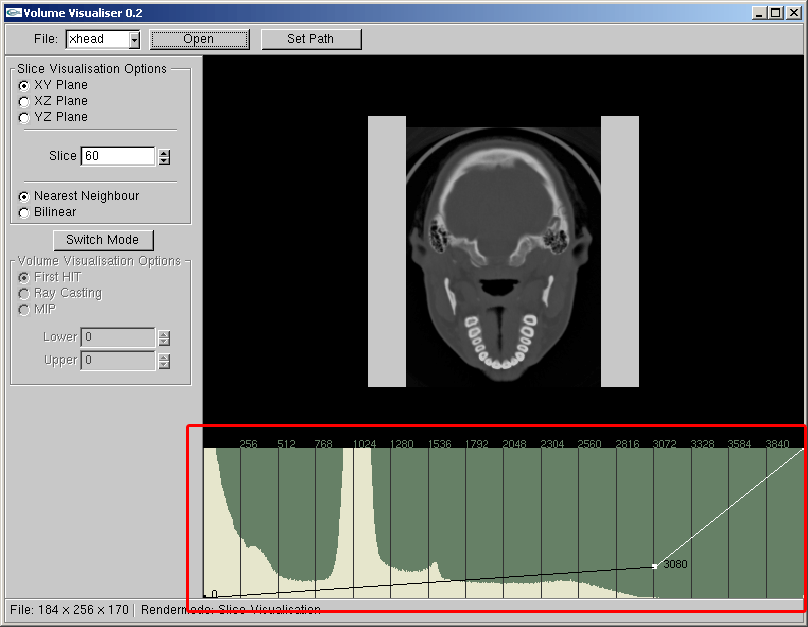
A white colored control point at density value 3080.
The user can also add a specific color by right click on an already defined control point. The right click brings up the color cube. To rotate the cube, the user needs to drag the mouse with the right button pressed. To select a color the left mouse button is used. Note that the histogram get disbled (i.e it does not respond to user interaction) as long as the color cube is visible. Also note that the height of a transfer point is mapped to the alpha value.
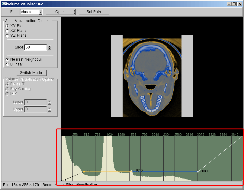
Added a blue colored control point at density value 1615 with the color selector cube beside (left). And a third control point in yellow for low densities (right).
It is also possible to delete slected controlpoints. To delete increasingly, select the leftmost point and press DELETE on the keyboard.

last update 06.12.2005