

by Oliver Mattausch, Thomas Theußl, Helwig Hauser, and Meister Eduard Gröller
Project Duration: 2002-2003
Abstract
This paper presents several strategies to interactively explore 3D flow. Based on a fast illuminated streamlines algorithm, standard graphics hardware is sufficient to gain interactive rendering rates. Our approach does not require the user to have any prior knowledge of flow features. After the streamlines are computed in a short preprocessing time, the user can interactively change appearance and density of the streamlines to further explore the flow. Most important flow features like velocity or pressure not only can be mapped to all available streamline appearance properties like streamline width, material, opacity, but also to streamline density. To improve spatial perception of the 3D flow we apply techniques based on animation, depth cueing, and halos along a streamline if it is crossed by another streamline in the foreground. Finally, we make intense use of focus+context methods like magic volumes, region of interest driven streamline placing, and spotlights to solve the occlusion problem.Keywords: 3D flow visualization, illuminated streamlines, interactive exploration, focus+context visualization
Download the paper
Oliver Mattausch, Thomas Theu�l, Helwig Hauser, and Meister Eduard Gr�ller, "Strategies for Interactive Exploration of 3D Flow Using Evenly-Spaced Illuminated Streamlines", to appear in Proceedings of SCCG 2003, paper.pdf (722 kb)Figures in the paper
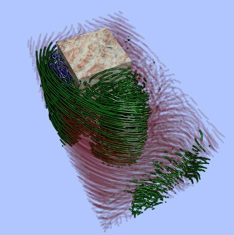 |
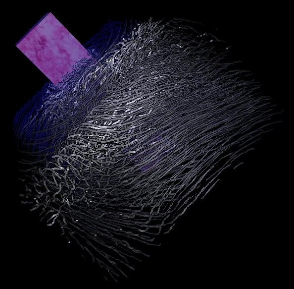
Figure 1: Flow around a block with high and low pressure coded as different colors and transparencies. |
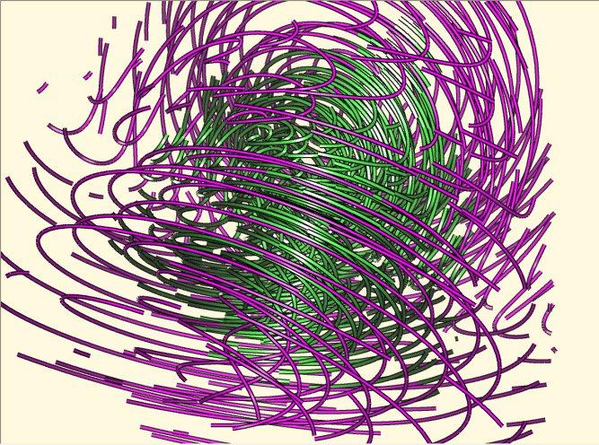 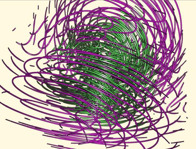 |
Figure 2: Lorenz system with focus region without end tapering (top) and with end tapering (bottom). Note the un-pleasing streamline endings at the focus region borders and streamline endings in general in the upper image. |
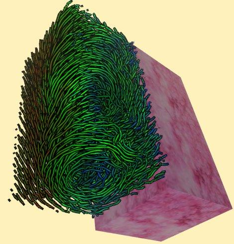 |
Figure 3: Color coded velocity with a continuous transfer function in the vicinity of the block. |
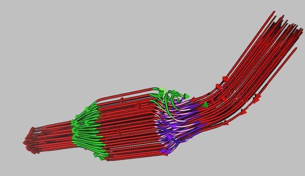 |
Figure 4: Catalytic converter with z-orientation as three scalar regions. Note the turbulence where the flow enters the converter. |
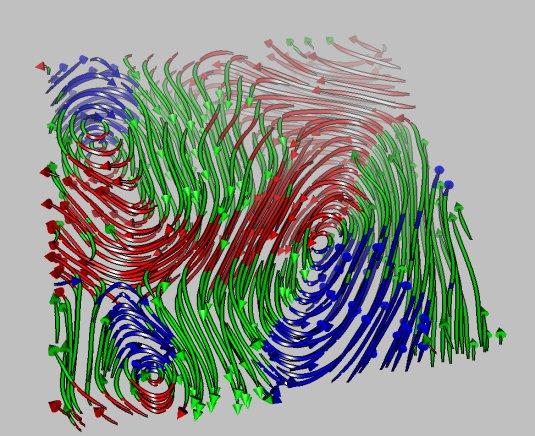 |
Figure 5: Smog over Europe, orientation in y-axis coded with 3 scalar interval regions. |
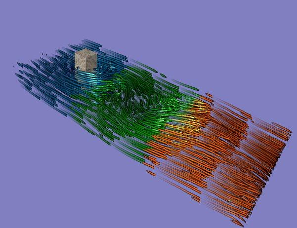 |
Figure 6: Flow around block with opacity function showing direction. Position in y direction is coded as scalar regions. |
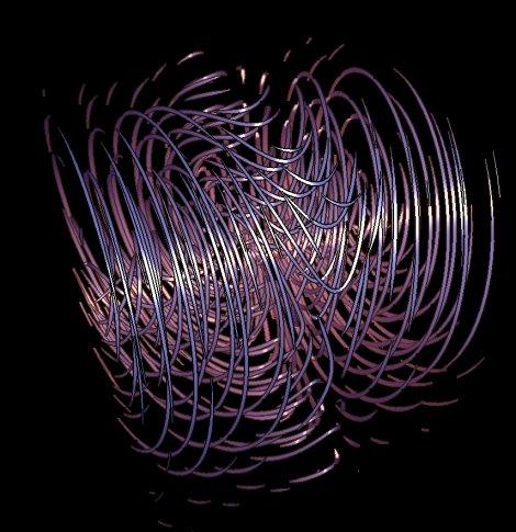 |
Figure 7: The Lorenz system with color coded depth. |
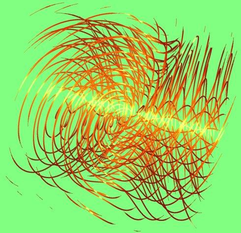 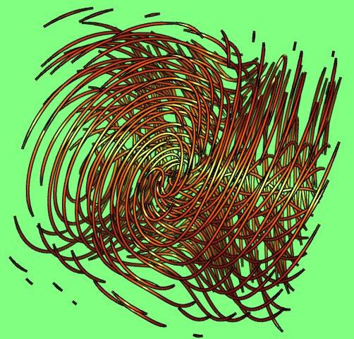 |
Figure 8: The Lorenz system without halos (top) and with halos (bottom). |
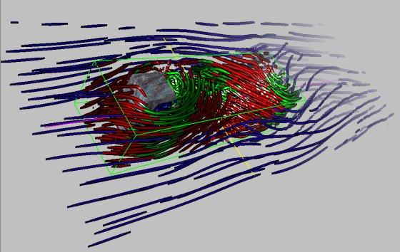 |
Figure 9: Flow around block with rectangular prism as magic volume (volume shown as geometry) and color coded pressure. |
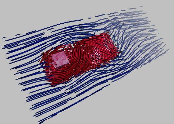 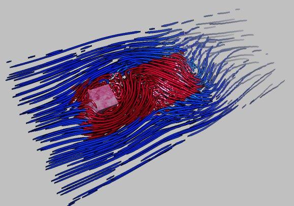 |
Figure 10: Flow around block with sharp border magic volume (top) and smooth border magic volume (bottom). |
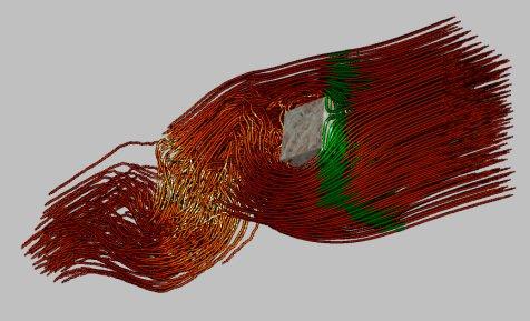 |
Figure 11: Magic volume used as seeding region (drawn green) in streamline calculation for the flow around block. |
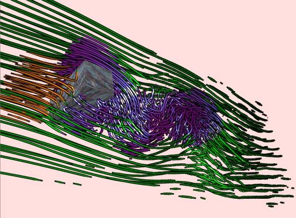 |
Figure 12: Flow around a block with three interval regions and pressure mapped to streamline density. |
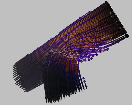 |
Figure 13: Spotlight shining on the t-junction data set. |