DESCRIPTION

MANUAL

APPLET

EXAMPLES

(Example definition file: cj.txt)

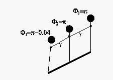
At first the simulation of the behavior of a number of coupled pendula is discussed. This system describes the mechanical dynamics of pendula, which can also be observed with SQUIDs (Superconducting Quantum Interference Devices) and  charge-density waves. The model of 2 torsionally coupled pendula

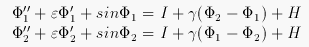
describes the behavior of the angles , which are damped by . I defines the constant bias current,  is the coupling of neighboring pendula and H is proportional to the applied magnetic field. In the following it is assumed that there is no forcing (I=0), no applied magnetic field H=0 and the coupling factor  is 0.1.

Due to the complexity that grows very fast with the number of pendula, it is mathematically hardly possible to investigate the evolution of systems with more than 2 pendula, although the set of equilibria often can be determined. The approach to approximate a system numerically  allows to simulate the evolution of one specific system with given starting angles and parameters.
 
 

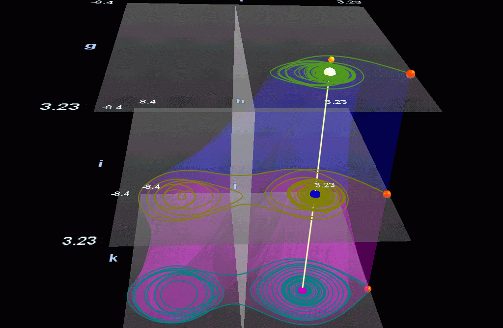
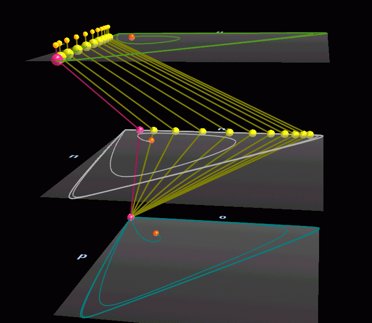
(a)	(b)	(c)

In (a) all pendula point exactly straight upwards. Only the first is rotated slightly, so that it slowly starts to pull down the other two pendula. By this the energy of the pendula's position is transformed into kinetic energy which causes intense motion. In contrast to the first case, these pendula are damped =0.1. Figure (b) shows a TDC plot where the angle of each pendula is plotted together with its derivation onto one plane. The second and the third pendulum intermediately are rotated over -PI and ''fall'' into another phase, but later on they return back into the origin phase where -PI<<+PI). The white cutting plane shows the phase change at -PI, and the marking polygon outlines the equilibrium to which the damped system finally converges.

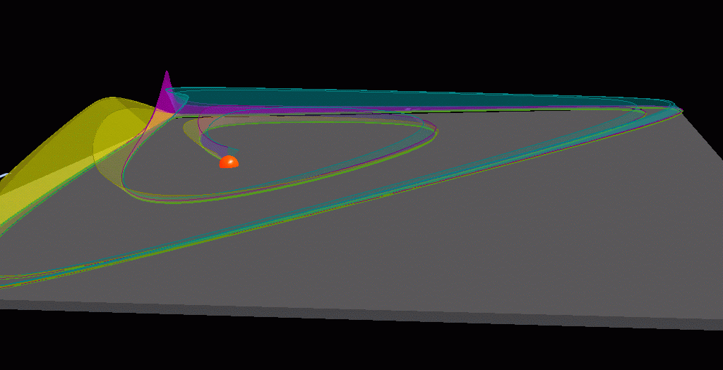
The EPC plot in figure (c) shows the evolution of a system with 5 pendula, where the rear 4 pendula start in position =0, and the first is initially rotated once (=2*PI). After a short time all pendula are affected and temporary a pendulum is rotated over -PI (upright position) into another phase.
 
 

(Example definition files: shg5.txt, shg6.txt and shg8.txt)

In the field of prebiotic evolution often dynamics are investigated, which shall describe possible chemical processes before life developed. An example for the simulation of the self-reproduction of polynucleotids is the symmetric hyper-cycle:

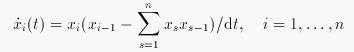
Observing the equation it can be seen that one equilibrium is given when all  are 0. For the simulation of a reproduction this fixed point is not relevant, whereas always a basic number should be existing. Concerning the term within the braces it can be experienced that it is only 0 at , which appears to be the only critical point.

Now the system is visually investigated with n > 4. The initial states are chosen near the equilibrium at . In fig. (a) the evolution of the system with 8 variables is shown using EPC. Observing one single variable it can be seen that periodically appearing peaks  alternate with periods of value 0. This phase is shifted from one variable to the next  constantly. More exactly, the value of the  raises at this time, when  leaves the peak. Then  passes over to 0 and stays there, until its preceding variable, i.e. , leaves its peak. It should be noticed, that  is  the predecessor of . By varying the starting vector, the system still falls into this cycle, whereas it can be called an attractor.
 
 

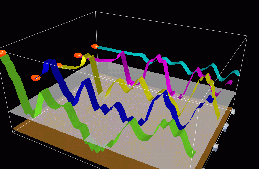
(a)	(b)	(c)

Another view of the cyclic behavior is given in fig. (b). The plot of the system with n = 5 using LWW shows a triangular trajectory on the base plane defined by  and . The values of the remaining 3 variables are  mapped into the length of the yellow, pink and cyan wing. Soon the trajectory ends up in the attracting cycle with the shape of a triangle. Here the characteristics of the cycle already outlined with EPC can be determined, too. The diagonal of the triangle represents the section, where the value of  raises while  falls. When  has reached 0,  starts to decrease and  to increase (yellow wing). In the corner (==0), the trajectory remains until  (cyan wing) starts to leave its peak.

Because of the homogeneous kind of the variables it is not a good aspect, that 2 variables have to be selected, which get a particular position in the visualization with LWW. But nevertheless all information can be obtained.

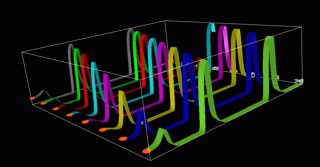
In fig. (c) a 6 dimensional trajectory is visualized with TDC. Starting at time 100 (red marker), 10 further markers with the same interval are inserted. In this period the second variable decreases, while the third variable grows. It can easily be seen that the other 4 values are 0 and do not change. The distance between the markers determines the speed of the trajectory, what shows that the trajectory slows down when an extremum is reached.