|
|
|
|
|
|
Introduction
|
|
This application has been developed in the course of the Visualisierung LU during winter term 2007/2008.
It enables you to visualize volumetric data for example from CT or MRT scans and is based on the paper Display of Surfaces from Volume Data von Marc Levoy [1].
|
|
|
|
|
Graphical User Interface (Overview)
|
The main window basically consists of up to 3 panels:
- rendering panel: here you can see the result of the visualisation
- control panel: allows you to load datasets, define the type of rendering, etc. (will be explained later on)
- transfer function panel: used for creating a transfer function (for certain 3D rendering modes)
|
|
|
Load/Save
|

- Load 3D Dataset: allows you to load 3D datasets of type DAT and DDS
-
Save Image: save an image to a file (JPEG)
- Aspect Ratio: you can chose between 4:3 and 16:9
- Resolution: 320 up to 2048 pixel (horizontally)
- Load/Save Transfer Function: gives you the possibility to save your current transfer function to a file and reload it later on
|
|
|
Rendering (2D)
|
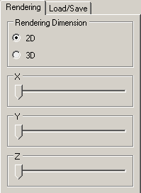
In 2D mode you can navigate through the volume by stepping through the individual slices along the main axes (x, y, z).
- X: slicing along the x axis
- Y: slicing along the y axis
- Z: slicing along the z axis
|
|
|
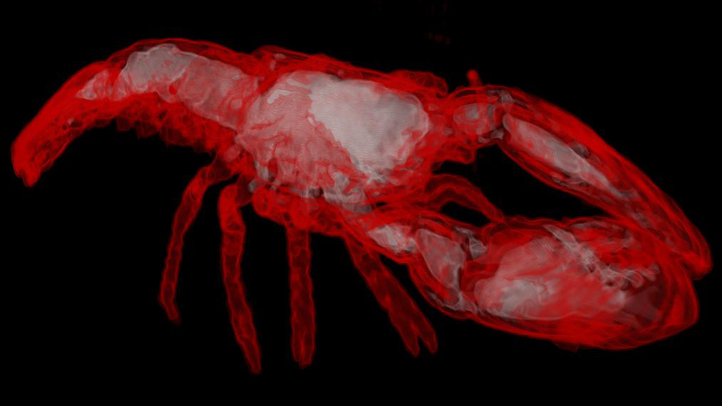
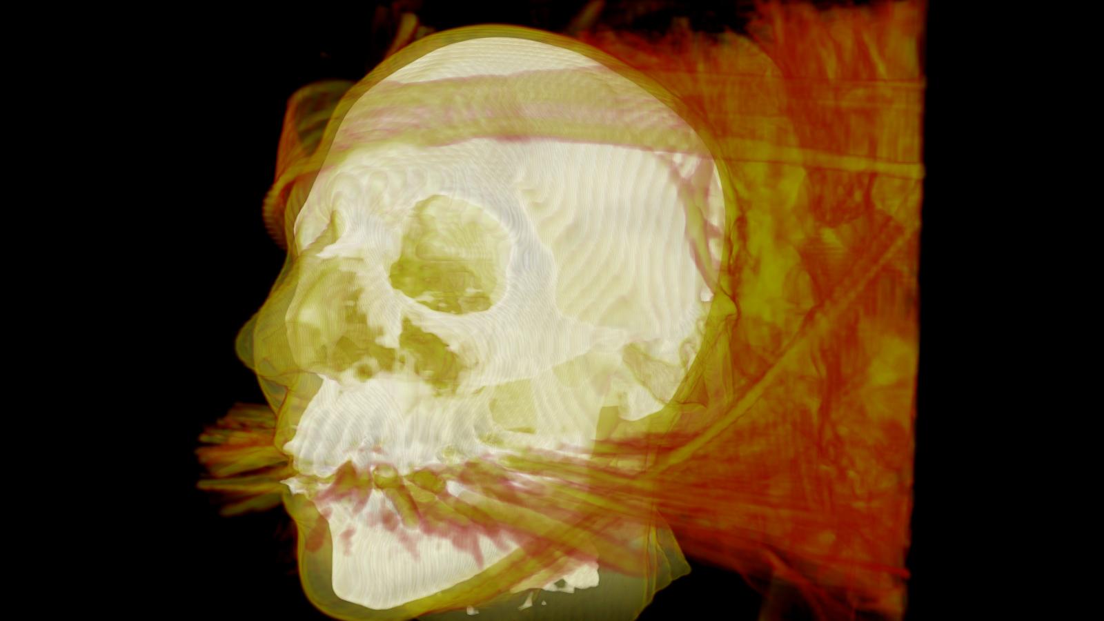
Rendering (3D)
|
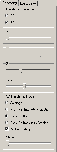
In 3D mode you can view the volume from an arbitrary angle. By using the sliders you can rotate the volume around the corresponding axis.
- X: rotation around the x axis
- Y: rotation around the y axis
- Z: rotation around the z axis
- Zoom: used for moving the volume closer to or further away from the viewer
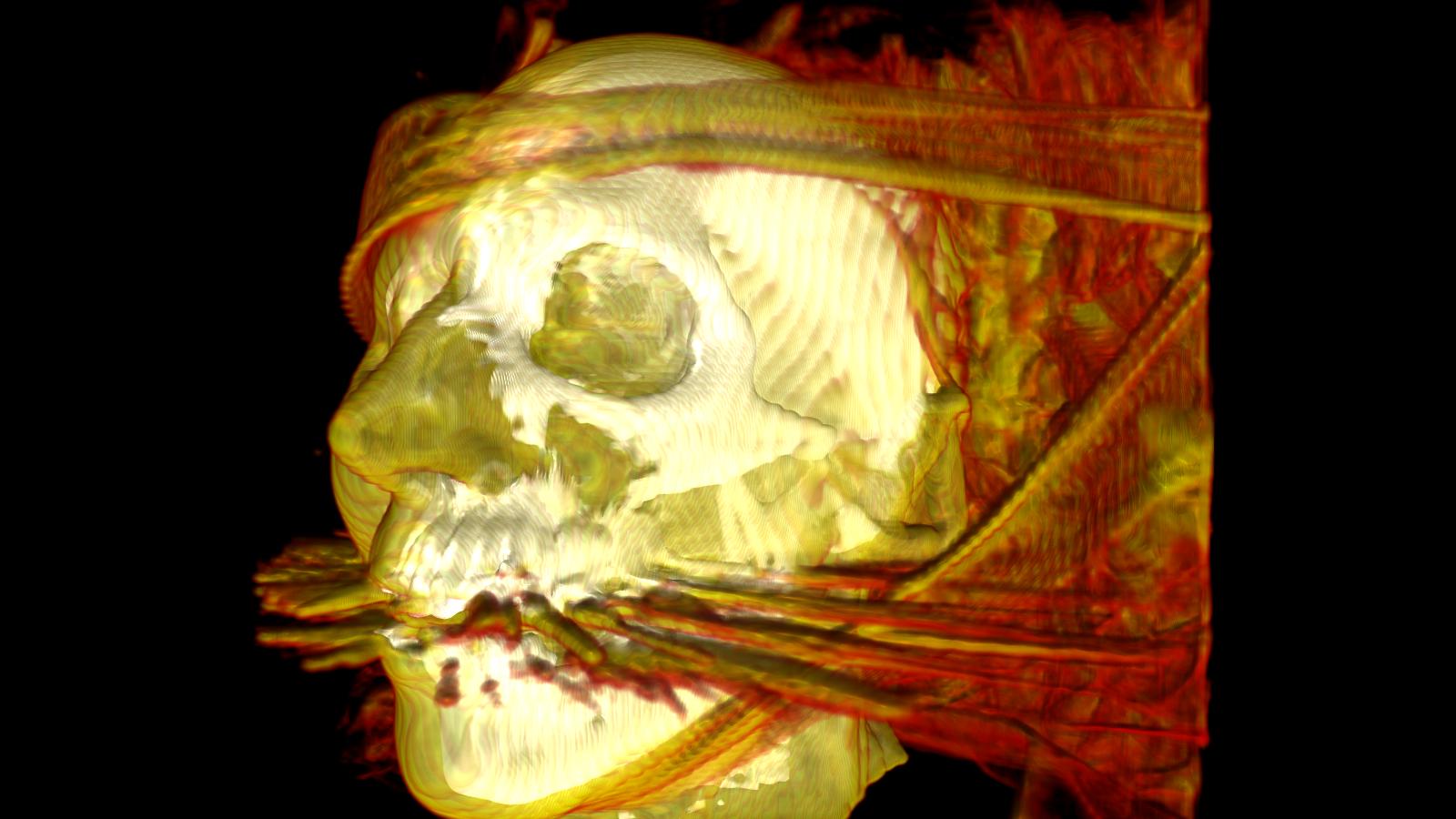
The possible rendering modes are:
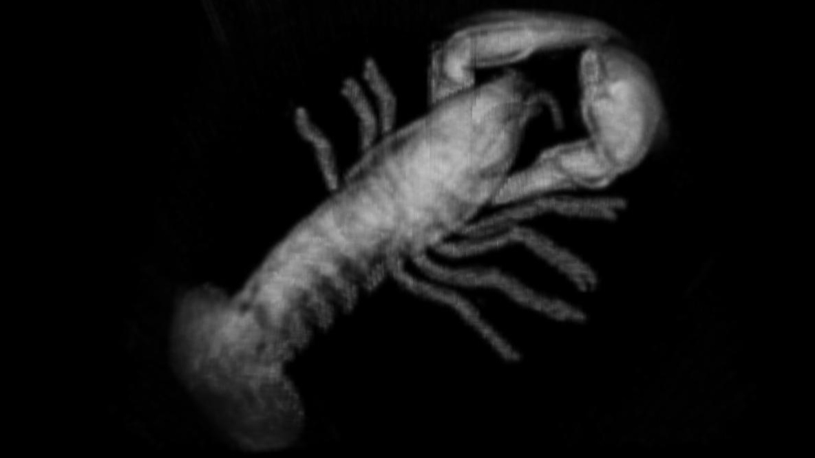
- Average (AVG): each voxel along the viewing ray is added equally weighted to the output pixel value(excluding the empty voxels)
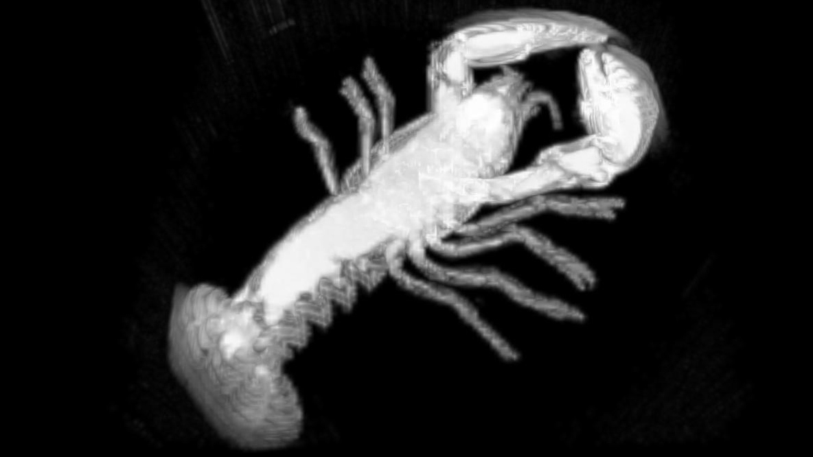
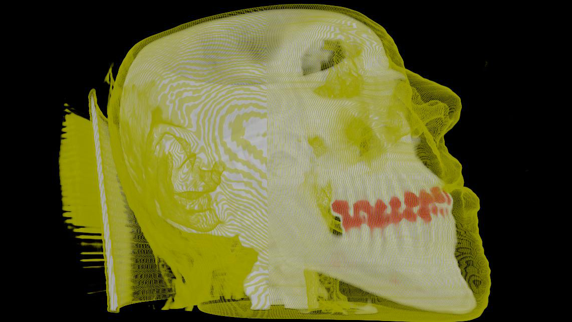
- Maximum Intensity Projection (MIP): the maximum value along the viewing ray is chosen as the output pixel value
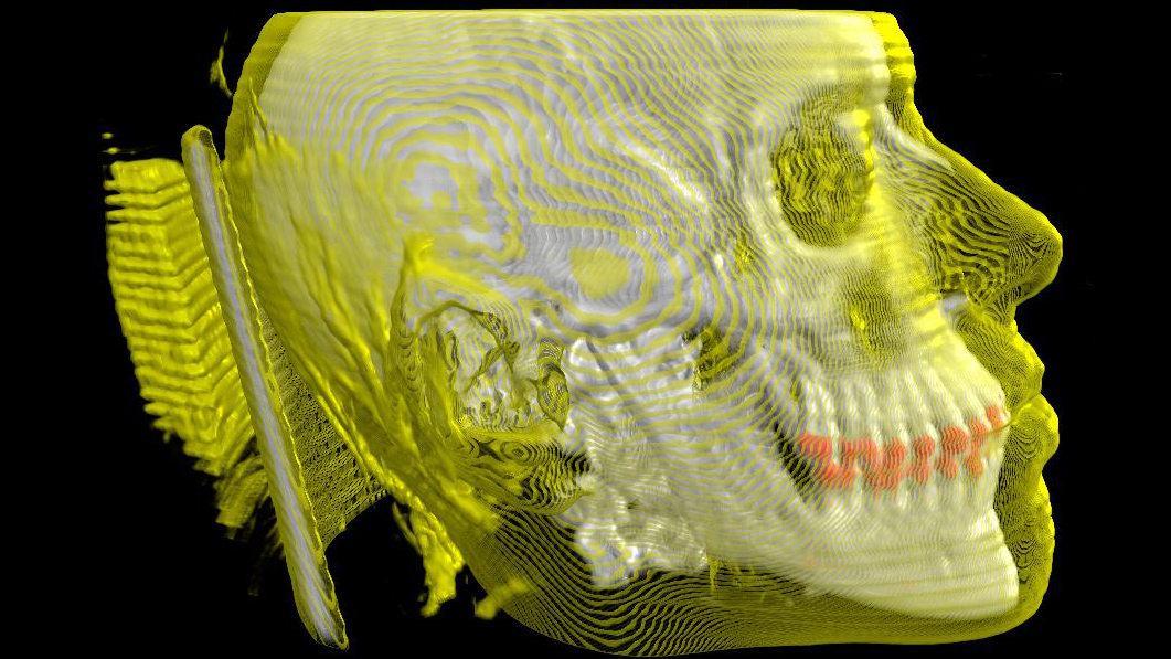
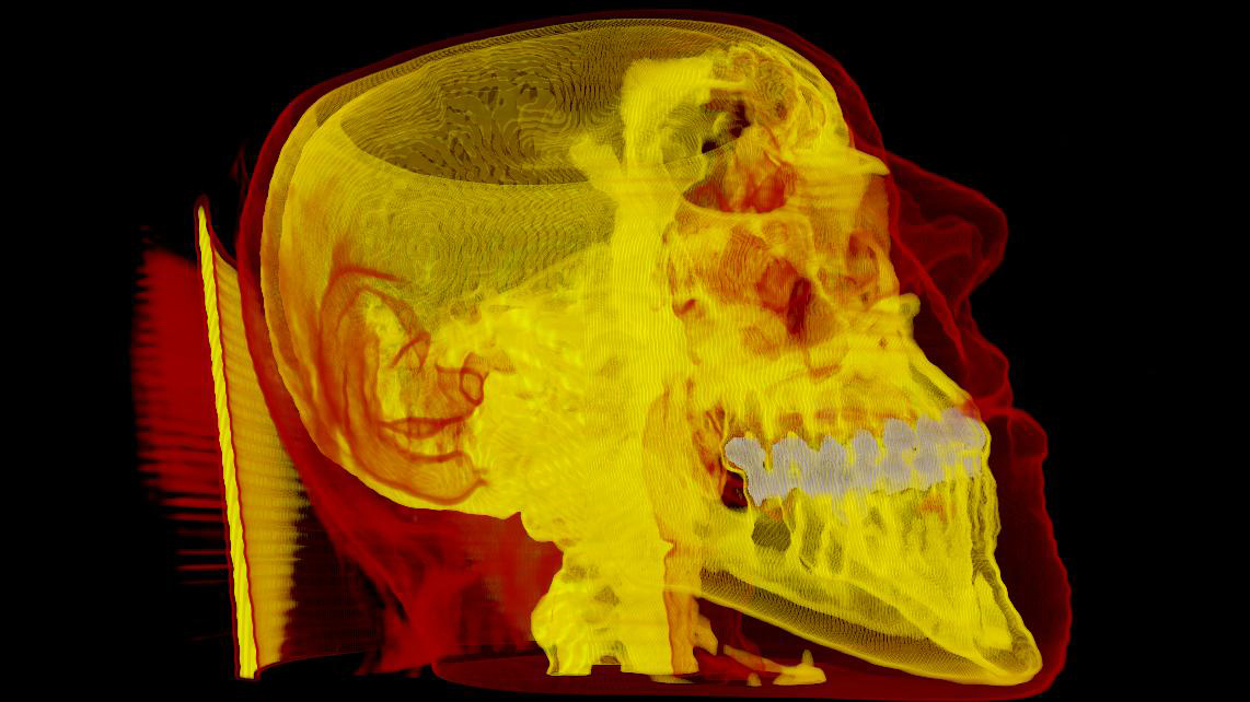
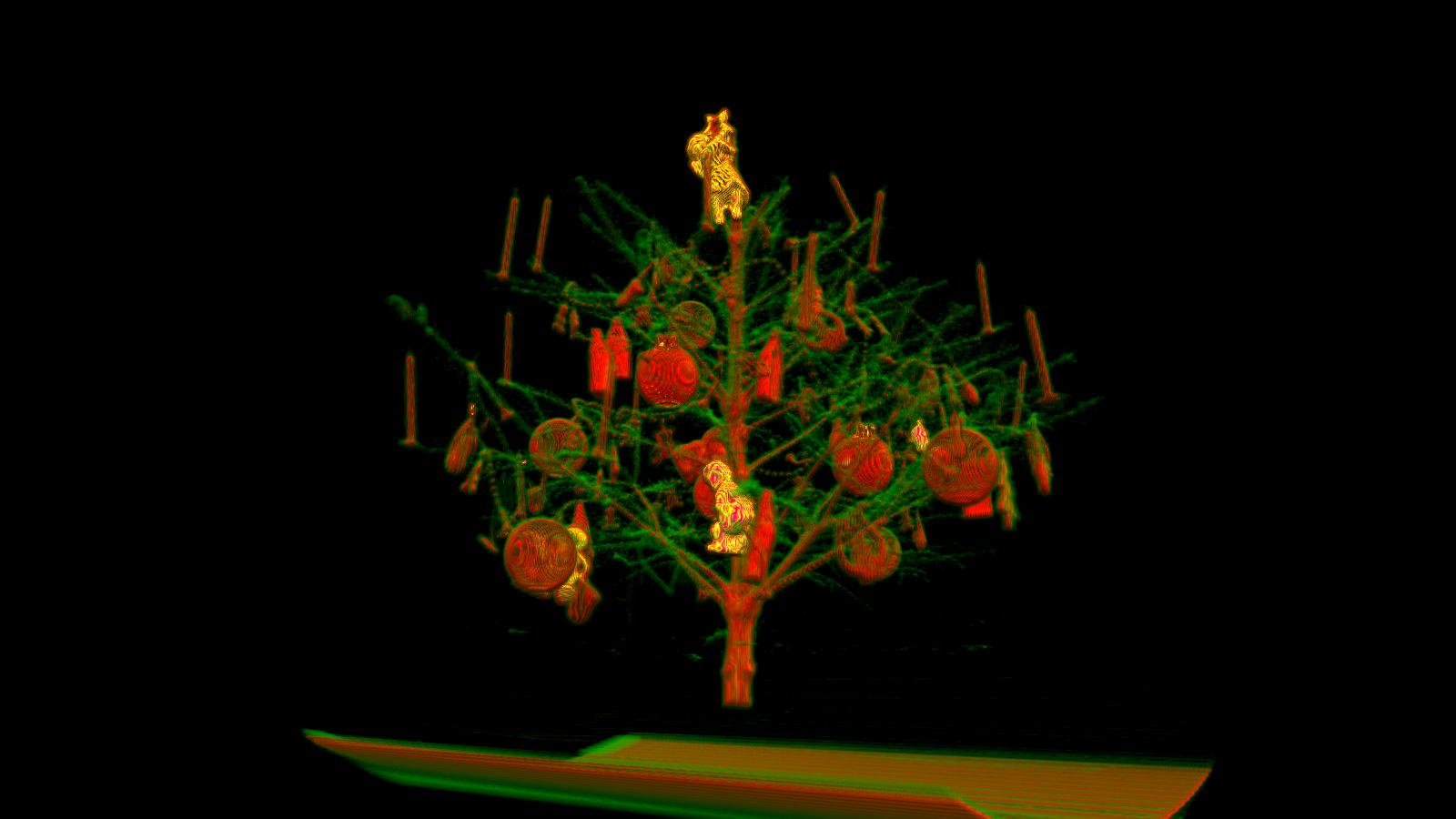
- Front To Back (FTB): by stepping through the volume along the viewing ray subsequent voxels contribute less and less to the output pixel color because they are obscured by the accumulated opacity of the previous voxels
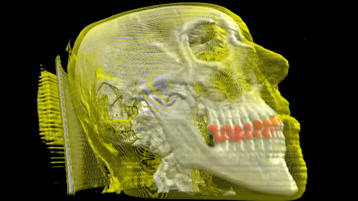
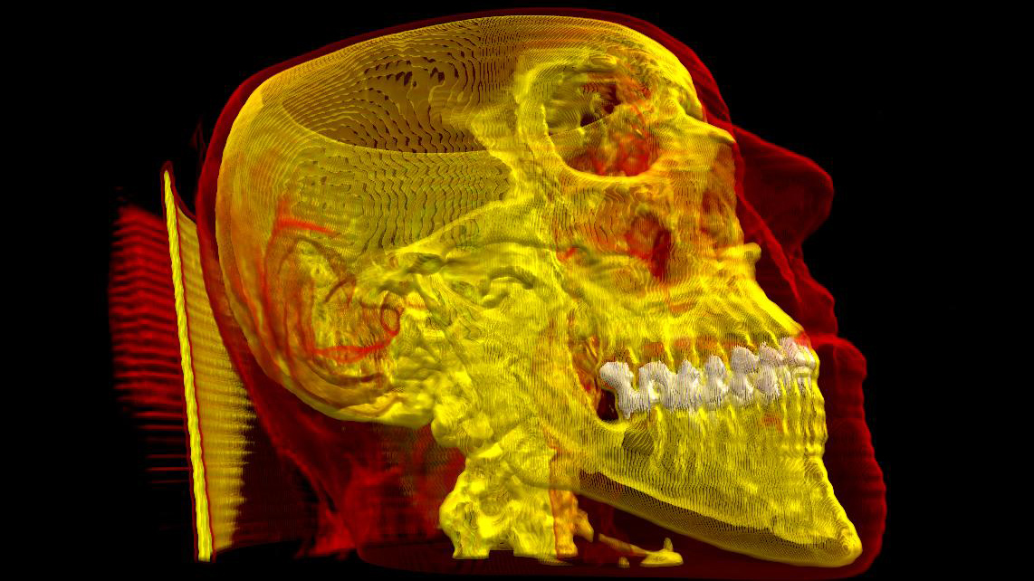
- Front To Back with Gradient: additionally to the iterative damping the gradient information is extracted and used as the normal vector for shading with the pong model
- Alpha Scaling: can only be used in combination with FTB and FTB with Gradient rendering mode
- Steps: lets you adjust the number of steps during sampling process along each viewing ray. By using more steps, the final result looks better but decreases the performance.
|
|
|
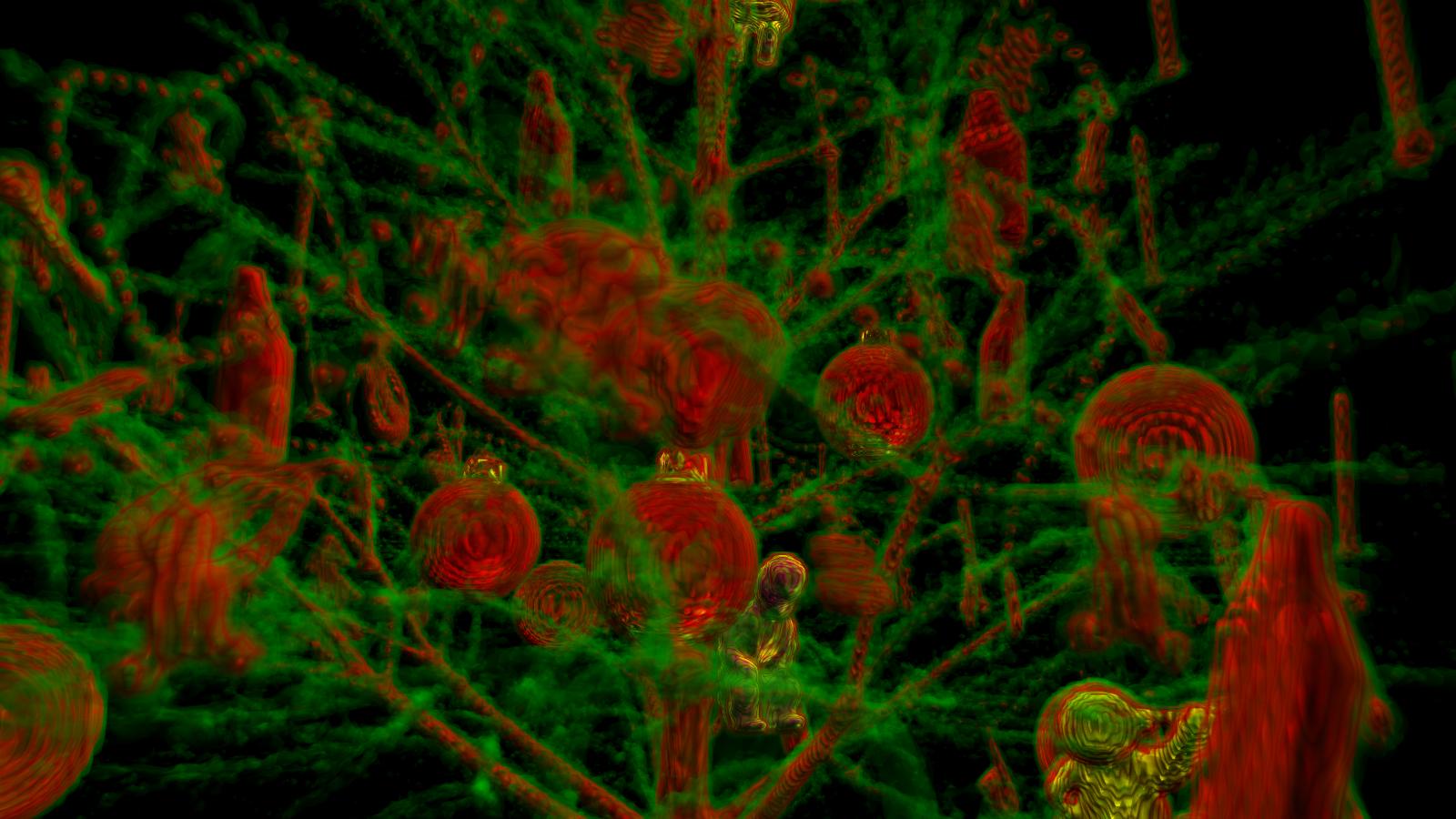
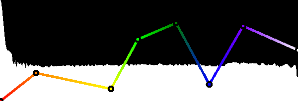
Transfer Function
|
|
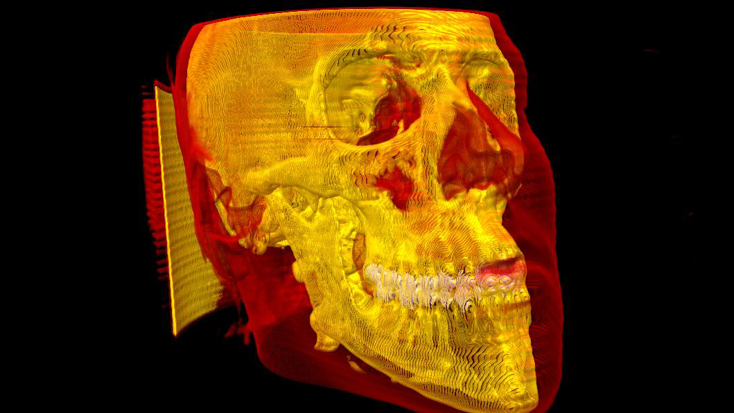
In the 3D rendering modes FTB and FTB with Gradient you have the possibility to define a transfer function wich is used for mapping the volume data value to color and associated opacity values.
- Clicking with the left mouse button into the histogram area (also the black part) you can put a point onto this position
- By using the "drag & drop" method you can change the position of the the point. Simply click on a point, hold the mouse button pressed and then move the mouse. When you release the button again the point is set at the new location.
- Double clicking onto a point opens a window where you can define its color.
- Clicking with the right mouse button onto a point removes it from the transfer function and its neighbour points are connected with each other.
|
|
|
|