Introduction
Example 2 was written for the "LU Visualisierung" at the Vienna University of Technology. It is a visualisation example for rendering flow visualisation images. It supports loading "*.gri" and the corresponding "*.dat" files. For a more detailed specification go here. There are four supported rendering modes, data grid, arrow plot, euler integration and runge kutta integration.
User Interface
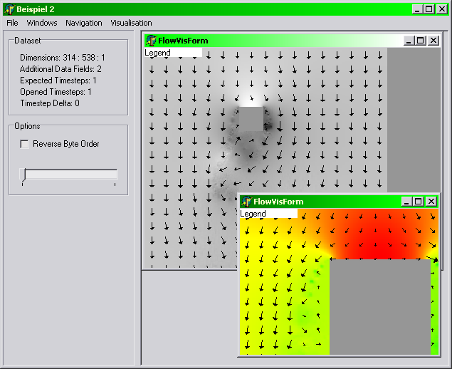
Beispiel2 is an MDI application, this means, multiple windows can be opened in one instance of Beispiel2. There can be only one opened dataset at a time, but different windows can show different modes of visualisation. It's up to the user to display as many child windows as he likes. An example of a possible workspace is shown below:
The following menus exist in Beispiel2:
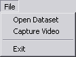
Open Dataset: Opens a grid file and the according data file.
Capture Video: Caputes a series of images in bmp-format corresponding to each timestep and saves them to the program's directory.
Exit: Exits Beispiel2.
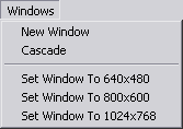
New Window: Opens a new visualisation child window.
Cascade: Cleans up the workspace by cascading all child windows.
Set Window To 640x480: Sets the main window's size to 640x480 (good for capturing).
Set Window To 800x600: Sets the main window's size to 800x600 (good for capturing).
Set Window To 1024x768: Sets the main window's size to 1024x768 (good for capturing).
These menus are specific for each child window:

Fit To Page: Fits the whole Dataset to the window.
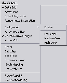
Data Grid: Renders the data grid to the window (one dot per gridpoint).
Arrow Plot: Renders an arrow plot to the window.
Euler Integration: Renders streamlines calculated with Euler integration to the window.
Runge Kutta Integration: Renders streamlines calculated with Runge Kutta integration to the window.
Background: Opens the submenu for background rendering.
Enable: Toggles background rendering.
Low Color: Sets the color for the minimum pressure of the dataset.
Med Color: Sets the color for a pressure of zero.
High Color: Sets the color for the maximum pressure of the dataset.
Arrow Area Size: Sets the size of a square which contains exactly one arrow (in pixels).
Variable Arrow Length: Toggles variable arrow length according to the length of the vectors in the dataset.
Arrow Color: Brings up a color dialog to choose a color for drawing arrows.
Set dt: Sets dt, the integration step size.
Set dSep: Sets dSep, the default distance for new lines.
Set dTest: Sets dTest, the minimum distance to other lines.
Streamline Color: Brings up a color dialog to choose a color for drawing streamlines (applies to both, Euler and Runge Kutta).
Glyph Mapping: Toggles glyph mapping on streamlines (small triangles which show the direction of the flow).
Set Glyph Size: Sets the size of a glyph relative to dt.
Force Repaint: Enable this if you have problems with repainting the window's client area. May cause flickering though.
2x2SS Antialiasing: Renders all images with double resolution and scales them down to achieve better image quality (looks nice, but degrades performance severely).
Navigation
The user can navigate the visualisation in two ways:
- Keyboard: By using the cursor keys the user can pan the dataset. By using + or - the view can be zoomed.
- Mouse: The user can pan the view by clicking and holding the right mouse button and dragging the mouse. When holding the left mouse button, the user can draw a rectangle, which will be zoomed to, when the mouse button is released.
- If the user is lost, he or she can return to the default view by selecting "Navigation->Fit To Page" from the menu.
Visualisation
Beispiel2 supports four rendering modi:
- Data Grid: Every dot represents one point in the underlying grid. Useful for checking how fine the grid is in different areas.
- Arrow Plot: A grid of evenly spaced arrows are drawn into the window. Each arrow's size corresponds to the underlying speed value. This behaviour can be disabled in the menu, to show arrows of equal size.
- Euler Integration: Euler is one method to visualise evenly spaced streamlines. The streamline is created point by point from the underlying grid. A valid seedpoint starts a streamline at a specific position in the grid. We fetch the vector at this point and move a little bit (dt) in that direction, so we get a new point. This procedure is done till we reach a saddel point our leave the drawing space.
- Runge Kutta Integration: Euler can be very improper. Runge solves this problem, by fetching the new vector at dt * 0.5 position away from the starting point. In this version only Runge Kutta 2 integration is implemented.
Screenshots |
[click on image for big view] |
")
|

|

|
| Arrow plot (fixed and variable length) |
Euler integration (left: dt=0.1, dsep=0.5, dtest=0.5) (right: dt=0.1, dsep=0.4, dtest=0.5) |
Runge integration with glyph mapping (smaller dsep and dtest) |

|

|

|
| Arrow plot (variable length) |
Runge integration (dt=0.01, dsep=0.3, dtest=0.2) |
Arrow plot, Euler and Runge with glyph mapping |
 |
 |
 |
 |
 |
 |
 |
 |
 |
 |
 |
 |
 |
 |
 |
 |
 |
 |
 |
 |
 |
 |
 |
 |
 |