User interface Guide
Contents
Interface Components
The interface is designed to be as simple and intuitive as possible. It is made of the following components: the (1)Menubar, the (2)Option Panel, the (3)Statebar and the (4)Rendering Area. Some components are only accessible at certain states of the program and will be described later.
Standard UI Components
(1)Menubar, (2)Option Panel, (3)Statebar, (4)Rendering Area.
The menu bar provides the functionality to load serveral *.gri files - which contains the geometry for a flow. If the program does not find any valid data file in the /data subdirectory, the user is only able to set a path. The path determines where the program should search for files and is given relative or absolute to the execution path. If the path does provide any valid file or can not be found, the ann error message will appear.
Please note the the program expects to find a *.dat file in the same directory, wich contains the data of the flow. The dat belonging to a gri file, are loaded automatically.
Set Path Dialog. If the path is not correct, an error message will be shown.
Once the path is set (correct), valid *.gri files are extracted and their names are stored in a drop down list. The user can now select one of these names and press open. The program will then load the file - wich is shown in the statebar. Once the loading has finished, the program enters the arrow plot mode.
The option panel lets the user select between the two render modes: arrow plot mode and streamline plot mode.. Therefore the user needs to press the Switch Mode Button.
How to arrow plot
Once a dataset has been loaded, the user can visualise the flow using arrows. In this mode, the statebar shows the message Rendermode: Arrow Plot Mode and the upper part of the option panel is activated. The user can select the following options
- Uniform Arrows
- Non Uniform Arrows.
- The size of the Arrows
Each option takes effect immediatly in the rendering area. When uniform arrows is activated, all arrows have the same length and are drawn in a (pixel) distance defined by the gridsize spinner. When the option nonuniform arrows is selected, the length of the arrows is scaled by the velocity.
Active Options in Arrow Plot Mode.
How to use the streamline plot
In the streamline plot mode, the user has the following options:
- Selection of the integration method
- Define the integration stepsize
- Define the seperating distance between the streamlines (dSep)
- Define the min seperating distance between the streamlines (dTest)
- Draw the streamlines using glyphs
- Draw the streamlines using glyphs
- Enable an interactive seedpoint setting
- Zoom a specific part
Options in streamline plot mode
Editing the Transfer Function
Once a dataset had been loaded, the user can enable the background texture by clicking the responding checkbox in the option panel. The background texture maps the additional dataset values to colors. Since we tested the program with the box dataset, there are two additional datasets available: the pressure and the vorticity. Note that only one of both textures can be visible at the same time
.
The shape of the Transferfunction
The transferfunction for each dataset are controlled by the min, current and max spinners. The min and the max value are mapped to blue. The current value is mapped to red. Values in between are interpolated. Values out of this range are mapped to black.
Screenshots
Pre-Release Images (Box Dataset)
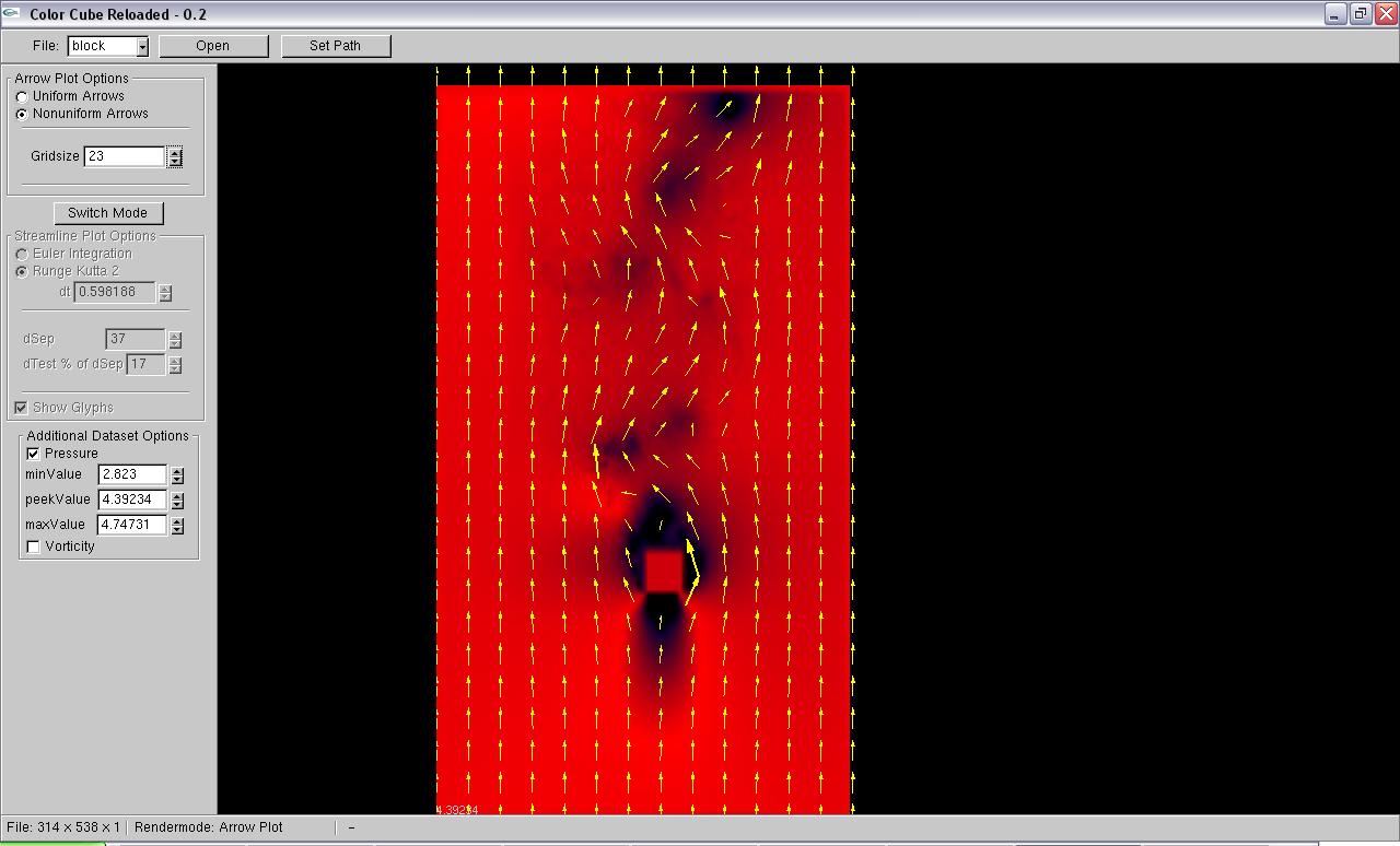
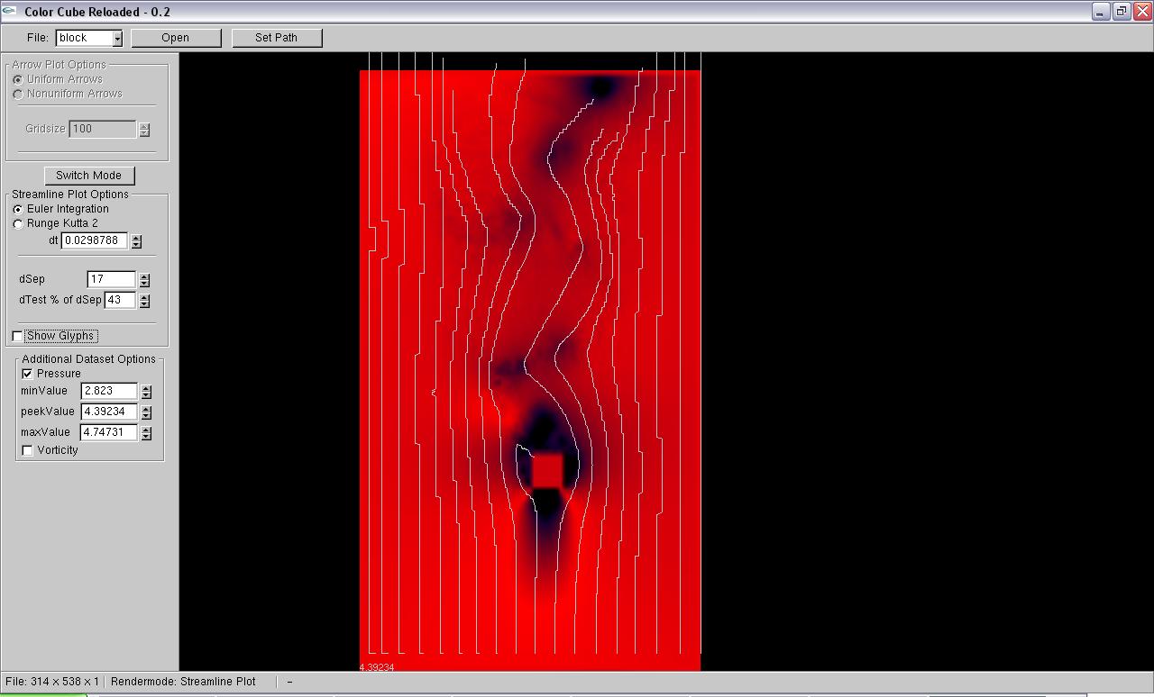
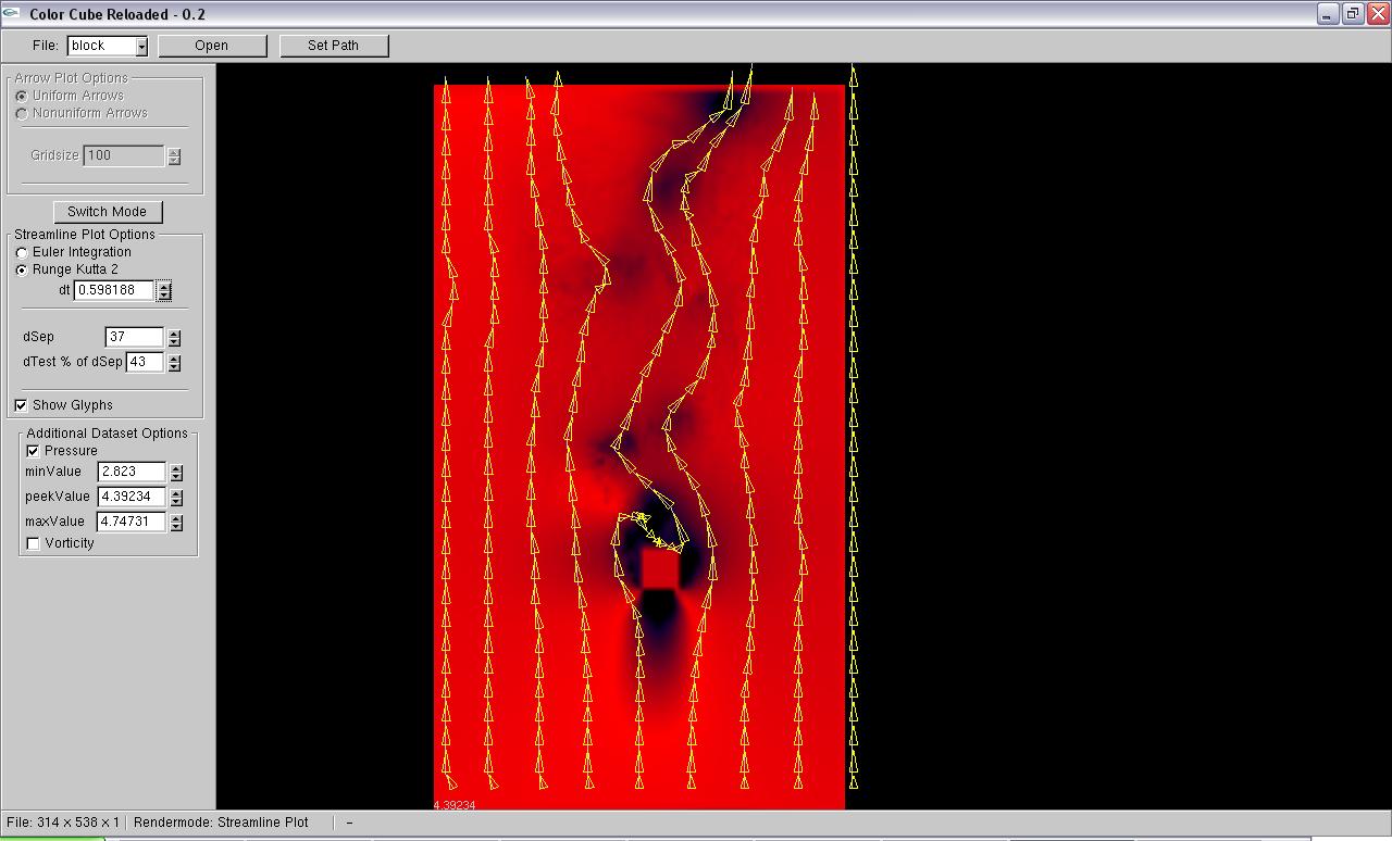
Images from the pre-release version. From left to the right: an arrow plot, a streamline plot, a streamline plot using glyphs. Note that the sampling in this version did not worked correct.
Final-Pre-Release Images (Box Dataset)


Composition
Final-Release Images (Box Dataset)
Texture Generation

last update 18.01.2006