CHARDIRS - visualizing eigen-manifolds

The first visualization technique presented here, i.e., CHARDIRS, is similar to the iconic representation of flow near critical points [31,74]. Instead of using a glyph to encode the flow topology, we directly represent the geometry of behavior by the use of stream lines and stream surfaces. We first inspect the eigenvalues of the Jacobian matrix and distinguish between topological different cases:

  

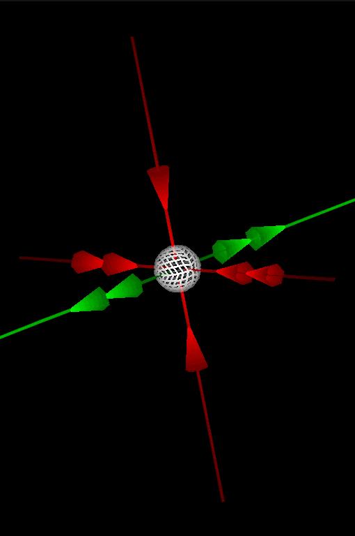
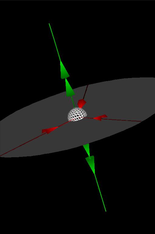
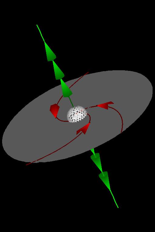
Figure 6.1: Visualizing the geometry of behavior near the critical point of a linear dynamical system - three different saddle configurations. [left image] [center image] [right image]

1.

If all the eigenvalues are real, different from each other, and different from zero, three pairs of stream lines are integrated into the direction of the corresponding eigenvectors. Thereby the (locally) most significant trajectories are depicted (see Fig. 6.1(a)).

2.

If all the eigenvalues are real, different from zero, but two of them are equal, a 1-manifold and a 2-manifold corresponding to the double eigenvalue build up the geometry of behavior near the critical point. In addition to a pair of stream lines we use three stream lines within the 2-manifold plus an optional stream surface to encode this special flow topology (see Fig. 6.1(b)).

3.

If two eigenvalues are complex and the real parts of all eigenvalues are different from zero, the same geometry of behavior is present as in the second case. Thus the same visualization technique is used (see Fig. 6.1(c)). However, the flow characteristics are different - spiraling vs. radial attraction/repulsion occurs.

To add more quantitative information we encode the order of magnitude of the eigenvalues by a certain number of arrows along the characteristic trajectories. Thereby the geometry of behavior near critical points is visualized for the most important cases. Degeneracies of flow geometry, e.g., non-hyperbolic critical points, are not considered through this approach.

  

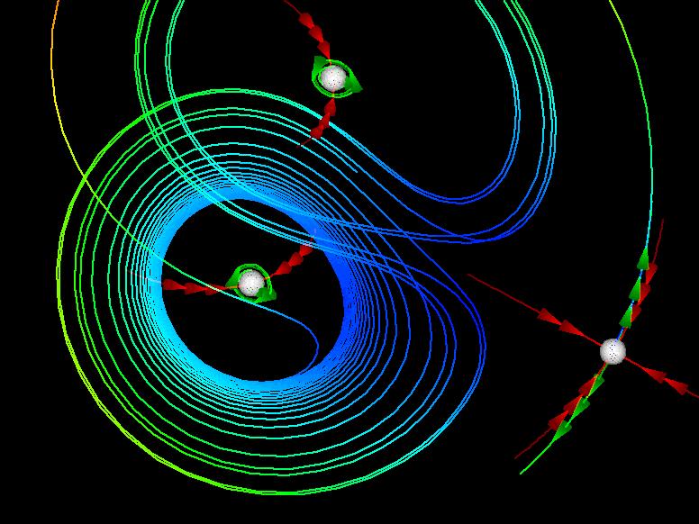
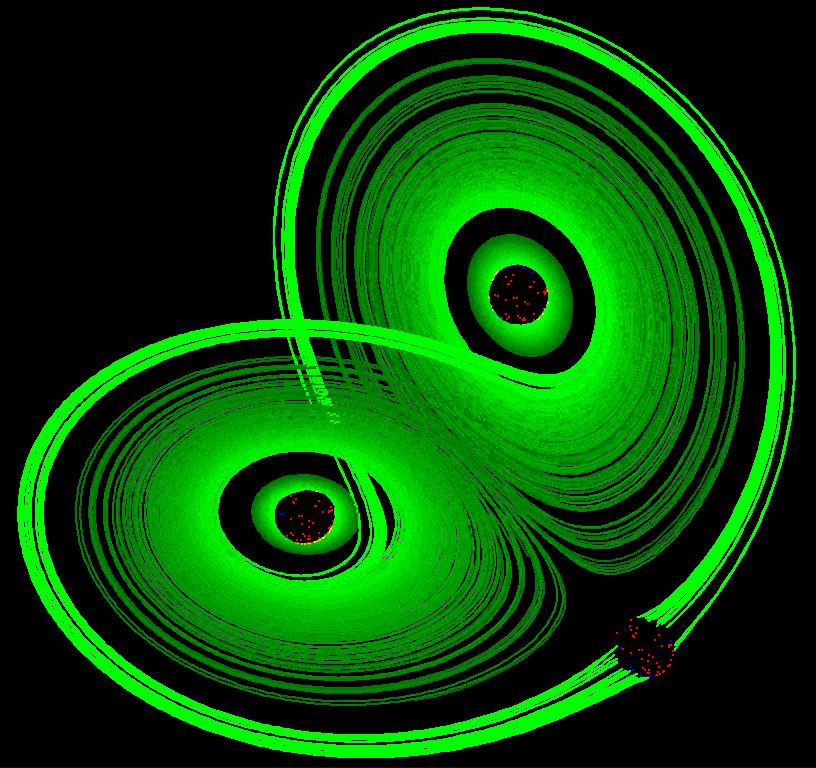
Figure 6.2: Visualizing the flow characteristics near the critical points of the Lorenz system:  (a) CHARDIRS and  (b) SPHERETUFTS.

In Fig. 6.2(a) the Lorenz system [63] was visualized by the use of this technique. Two saddle foci with (each) a pair of conjugated complex eigenvalues and a large negative real eigenvalue drive the rotating characteristic of this chaotic dynamical system. A third saddle coordinates the alternating dominance of these two foci.

mailto:helwig@cg.tuwien.ac.at.