Next: Dynamical systems Babylon of
Up: Notes on the local
Previous: Classifications of dynamical systems
The solution of a continuous dynamical system is a trajectory
 as defined by
Eq. 3.1 [40,69].
Any point on the
trajectory is given by its parameter t and an initial state
s of the system.
Parameter t can be interpreted as the time passed since the
system evolved from
s. Note, that Eq. 3.1 is
a ``recursive'' definition (integral equation) that cannot be
expressed explicitly in most cases.
as defined by
Eq. 3.1 [40,69].
Any point on the
trajectory is given by its parameter t and an initial state
s of the system.
Parameter t can be interpreted as the time passed since the
system evolved from
s. Note, that Eq. 3.1 is
a ``recursive'' definition (integral equation) that cannot be
expressed explicitly in most cases.
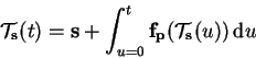 |
(3.1) |
Differential geometry includes the analysis of curves and surfaces
in higher dimensions.
The construction of a local coordinate
system (Frenét-Frame) helps to get insight into local
characteristics of a spatial curve, e.g., curvature and
torsion [10,30].
Local analysis of trajectories
requires a good working knowledge of various terms of differential
geometry.
They are shortly discussed in the following.
Given a parameterized curve
 in three-space a
re-parameterization is possible such that the curve's new parameter
s is equal to the arc length of curve
in three-space a
re-parameterization is possible such that the curve's new parameter
s is equal to the arc length of curve
 in the
parameter interval [0,s).
In respect to these distinct parameters derivations of curve
are written differently:
in the
parameter interval [0,s).
In respect to these distinct parameters derivations of curve
are written differently:
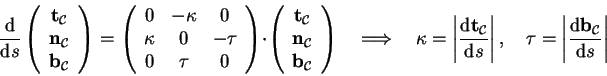
By the use of these derivations a local coordinate system
(Frenét-Frame) can be built at a curve point by the curve's
tangent vector
 ,
its
principal normal
,
its
principal normal
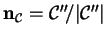 ,
and its binormal
,
and its binormal
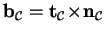 .
These three vectors span an orthonormal basis at a curve point. Note,
that
.
These three vectors span an orthonormal basis at a curve point. Note,
that
 and
and
 are
ambiguous when the curve is locally equal to a straight line.
are
ambiguous when the curve is locally equal to a straight line.
By building the Frenét-Frame at a point on the curve the
curvature  and the torsion
  of curve
at this point can be derived in a straightforward way from the
orthonormal basis [10]:
of curve
at this point can be derived in a straightforward way from the
orthonormal basis [10]:
Curvature
and torsion
of curve
can
be described in other terms as well. For example, the curvature
of a curve can be written as 1/r, when r is the radius of the
osculating circle [13].
As a third possibility,
can be derived by the following
procedure: assuming  to be the angle enclosed by the
curve's tangent and the line running through
to be the angle enclosed by the
curve's tangent and the line running through
 and
some point
and
some point
 ,
slightly ahead on the curve,
the curvature
can be calculated as
,
slightly ahead on the curve,
the curvature
can be calculated as
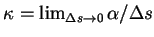 .
.
Torsion can be similarly derived by a differential quotient.
Assuming  to be the angle enclosed by a line through
and
the rectifying
plane (spanned by
to be the angle enclosed by a line through
and
the rectifying
plane (spanned by
 and
), the torsion
can be calculated
as
and
), the torsion
can be calculated
as
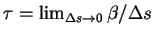 [13].
[13].
Next: Dynamical systems Babylon of
Up: Notes on the local
Previous: Classifications of dynamical systems
Helwig Löffelmann, November 1998, mailto:helwig@cg.tuwien.ac.at.