![\framebox[\textwidth]{
\begin{tabular*}{.93\linewidth}{@{}@{\extracolsep{\fill}...
...plex.2.ps}
\\ {\small{}(a)}
& {\small{}(b)}
& {\small{}(c)}
\end{tabular*} }](img248.gif) |
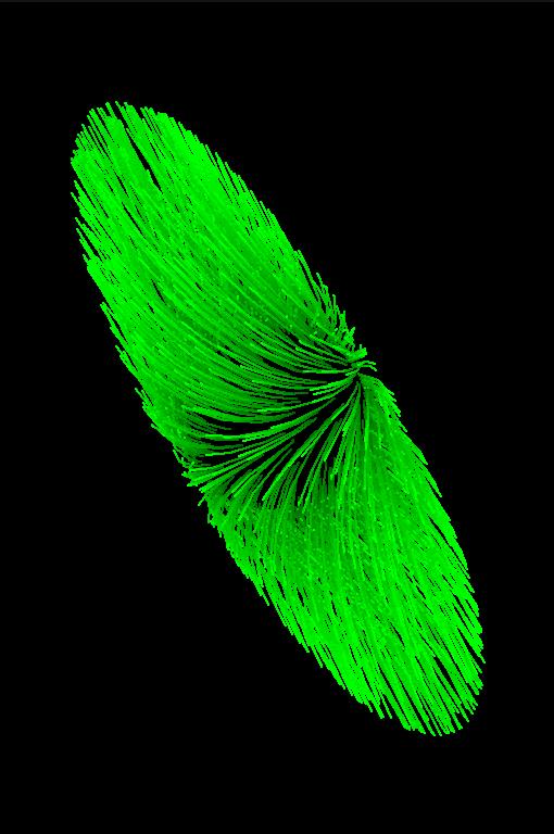
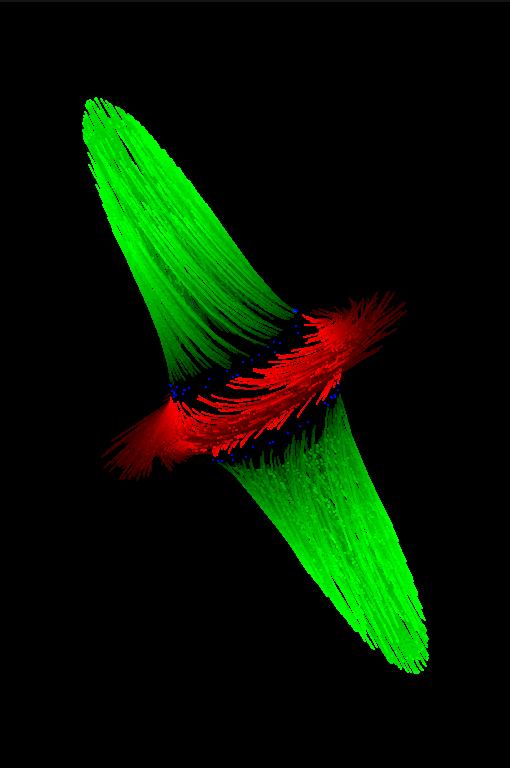
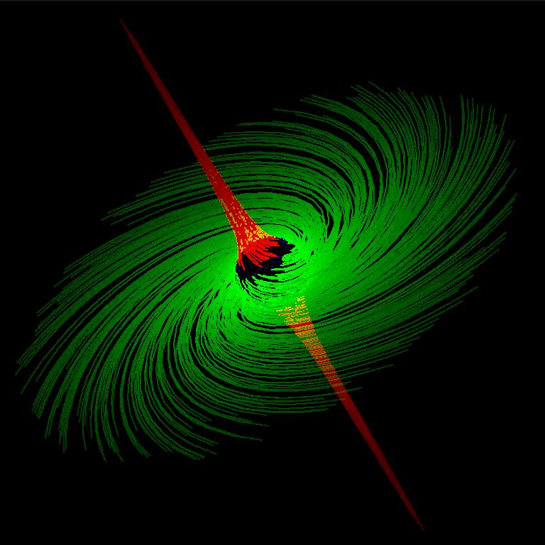
In Fig. 6.3 three examples are given. Fig. 6.3(a) shows a linear repellor focus, whereas Fig. 6.3(b) depicts the saddle focus of a linear dynamical system. Fig. 6.3(c) shows also a linear saddle focus as in Fig. 6.3(b) with different eigenvalues. Using this direct visualization technique subtle differences in the flow characteristics become visible. By the use of SPHERETUFTS the differences between Fig. 6.3(b) and Fig. 6.3(c) become visible, although the flow geometry is identical in both cases: the flow component related to the real eigenvalue is much stronger in Fig. 6.3(c) than in Fig. 6.3(b).
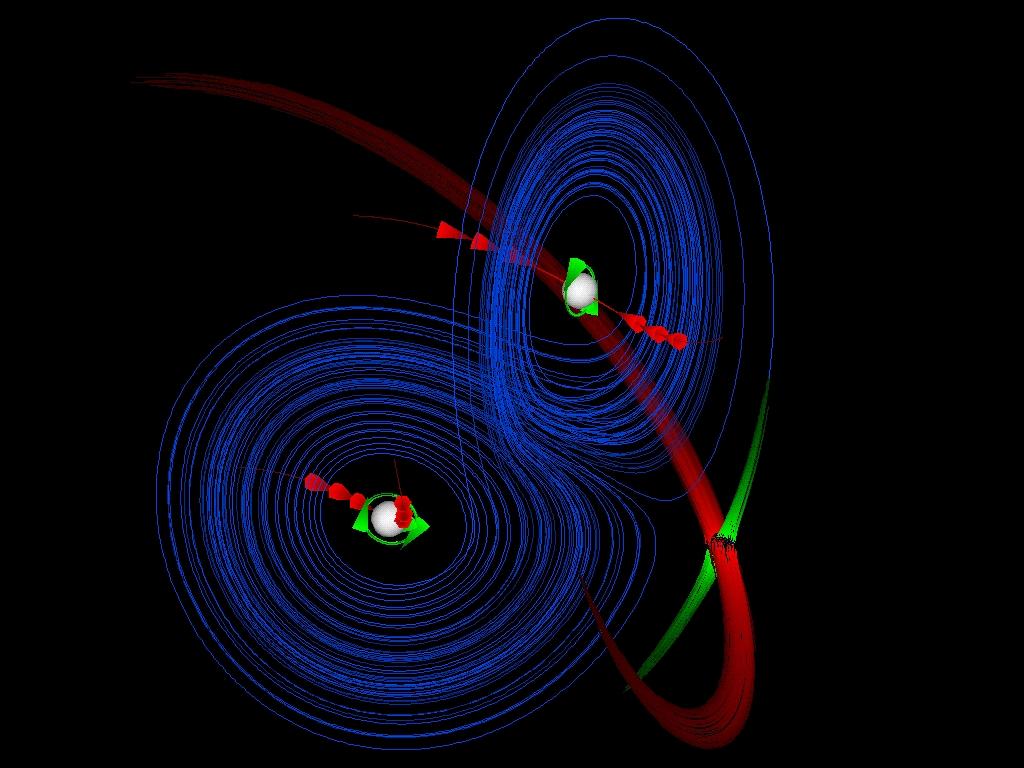
In Fig. 6.2(b) the Lorenz system was visualized by
placing bunches of streamlets near the critical points. The most
important flow characteristics are
intuitively depicted.
See Fig. 6.4 for a visualization of the Lorenz
system by the use of SPHERETUFTS and
CHARDIRS.
Although the results gained with this method are quite expressive,
the uniform distribution of streamlet seed points over a sphere
enclosing the critical point might not be the
optimal choice. Using a seed value distribution, which reflects the
distance to the characteristic directions, i.e., the
trajectories which coincide with the eigenvectors of the critical
point, the visualization can be improved.
![\framebox[\textwidth]{
\includegraphics[width=.93\linewidth]{pics/Lorenz-old.ps}
}](img249.gif)