For our explorations of parameter space of the Lorenz system, the parameters
 = 10, b = 8/3 remain constant. Only r, will be varied.
The following diagram illustrates the behaviour for small values of r:
(Because the Lorenz system is symmetric only one half of the bifurcation
diagram is displayed):
= 10, b = 8/3 remain constant. Only r, will be varied.
The following diagram illustrates the behaviour for small values of r:
(Because the Lorenz system is symmetric only one half of the bifurcation
diagram is displayed):
for r<1 the Lorenz system has only one attracting fixed point. It is the origin
C0 = (0,0,0) of the phase space.
C0 stands for no rotation of the waterwheel
i.e. any rotation stops after some time.
At r=1 the fixed point C0 looses its stability in a
supercritical pitchfork bifurcation.
C0 becomes a repellor and the system gets two new fixed points C+with x=y=+ , z=r-1 and C- (not shown in diagram) with
x=y=-, z=r-1.
, z=r-1 and C- (not shown in diagram) with
x=y=-, z=r-1.
At r=24.24 the fixed points C+ and C- loose stability by absorbing an
unstable limit cycle in a
supcritical hopf bifurcation.
When decreasing r, the limit cycles get larger until the cycles touch at r=13.926. Below r=13.926
there are no limit cycles. The waterwheel saddles in a steady rotation in either direction immediatly
independent of its initial condition.
Above r=13.926 the system exibits transient chaos. The waterwheel may change its direction
chaotically several times until saddles in a steady rotation (see images for r=19.0 and r=21.0 below).
Oberserving trajectories in phase space one can see, that trajectories being far away from one fixed point,
after changing the sign of x and y get near to the other fixed point
(it is the stretch-split-merge behaviour described in [Peit92]).
When a trajectoriy gets near enough (settling within the limit cycle), it is attracted to the fixed point.
Otherwise it is again repelled until x and y change in sign again and so on.
Above r=24.06 there is no more transient chaos and the system becomes a strange attractor. Trajectories
being outside a limit cycle can not get inside any limit cycle as it is the case for transient chaos. That is
because the limit cycles do not intersect with the attractor. Therefore trajectories on the attractor can not
get close enough to a fixed point C+ or C- to be attracted to it.
Only trajectories starting near enough a fixed point
(or specific other initial conditions that are not on the attractor) can be attracted to a fixed point
(see images for r=24.1). [Stro95]
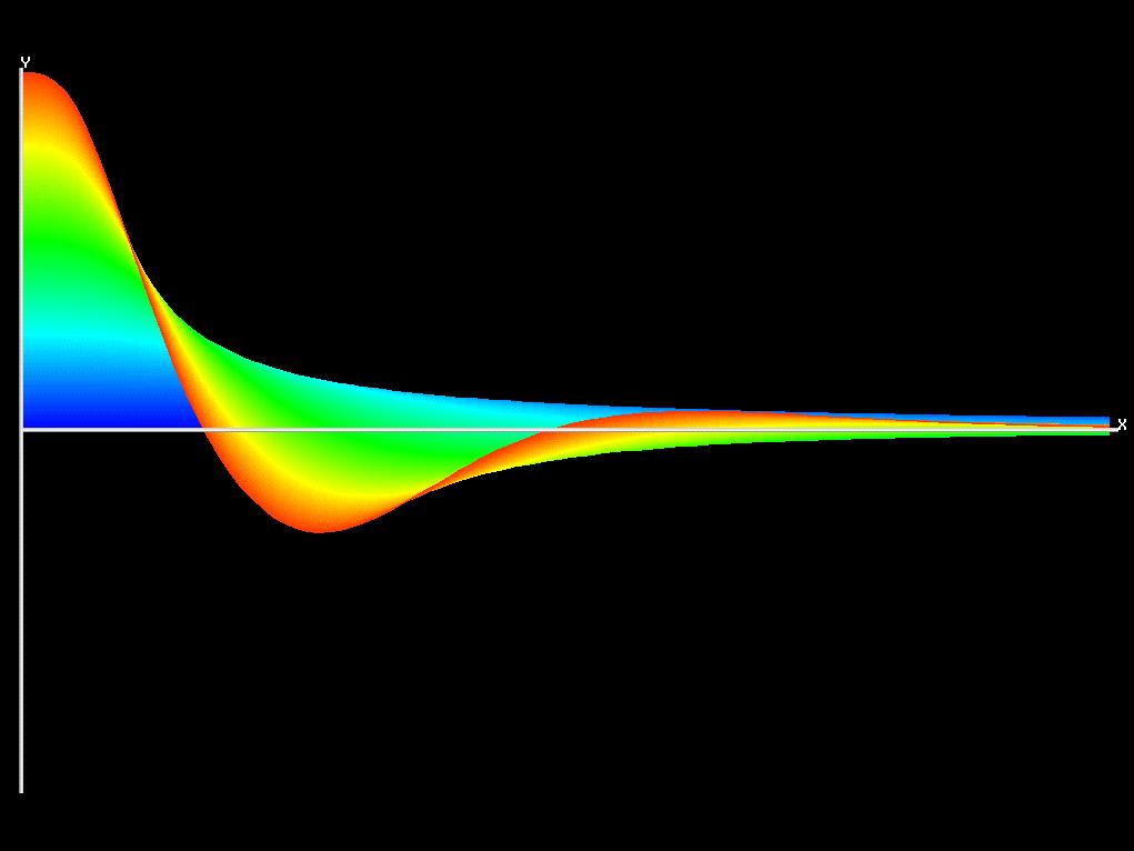
For visualizing the behaviour described in the above diagramm, it is
nescesary to observe the long time behaviour of many trajectories in
phase space. This can be achived by using two-dimensional diagrams.
Time is displayed along the horizontal axis. Along the vertical axis, the x-coordinate in
phase space of many trajectoriesis displayed (it is the rotation speed of the chaotic waterwheel
and the convection rolls in fluids or gases).
The initial points are distributed on a
line with startpoint (0, 0, r-1) and endpoint (L, L, r-1) where L was
chosen as 25 to cover a wide range of initial conditions. If r<1 then z=0.
The fixed points different from the origin of phase space are displayed as
light red tubes.
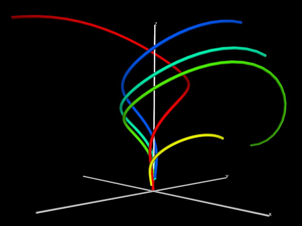
Another way for visalizing long time behaviour is to visualize trajectories in 3D phase space with different kinds of color-encoding of the trajectories.
Two different ways of color encoding are used.
The first is to encode the distance of the initial points of the trajectories to the
z-axis. This way of color coding allows to follow the path of the points
along the time axis and was applied to the 2-dimensional diagrams x(t).
The second way is to use color-coding for time. Blue trajectories are old and
yellow or red trajectories are young. This helps to recognize slow movements
from or to fixed points. This way of color-coding was used for
visualizing trajectories in phase space.
|
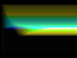
for r<1 the Lorenz system has only 1 attracting fixed point C0. It is the origin
(0,0,0) of the phase space. All trajectories are attraced to this fixed point
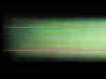
i.e any rotation stops after some time. Upper image (30K): r=0.5 and 100 iteration steps have been made. 600 starting points have been taken with a maximum distance of 35 (L=25) from the origin. Lower Image (42K): r=0.5, trajectories starting at different points in phase space being attracted to C0. Different trajectories have different colors for better distinction (Image has 42K). |
|
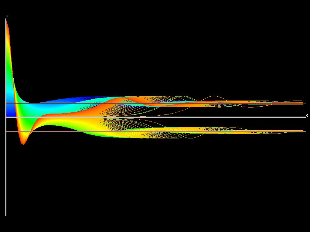
At r=1 the attracting fixed point looses its stability in a
supercritical pitchfork bifurcation
The attracting fixed point C0 becomes a repellor and the system gets two
new fixed points C+ and C- (see above). In dependence of initial points,
trajectories are attracted to either one of these two fixed points. In terms of the waterwheel
one can say that in dependence of the initial condition it ends in a steady
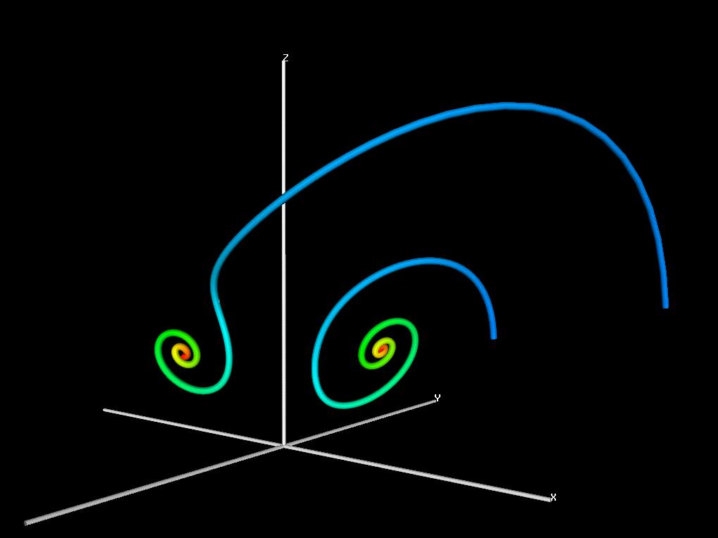
rotation in either direction. Upper image (51K): r=6.0, 500 iteration steps have been made. 500 starting points have been chose with a maximum distance of 35 (L=25). Trajectories are attracted to either C+ or C- Lower image (34K): r=6.0, two trajectories are being attracted to one of the fixed points C+ or C-, depending on the startpoint of the trajectory. Color-coding of time is used. The trajectories start blue and end red. |
|
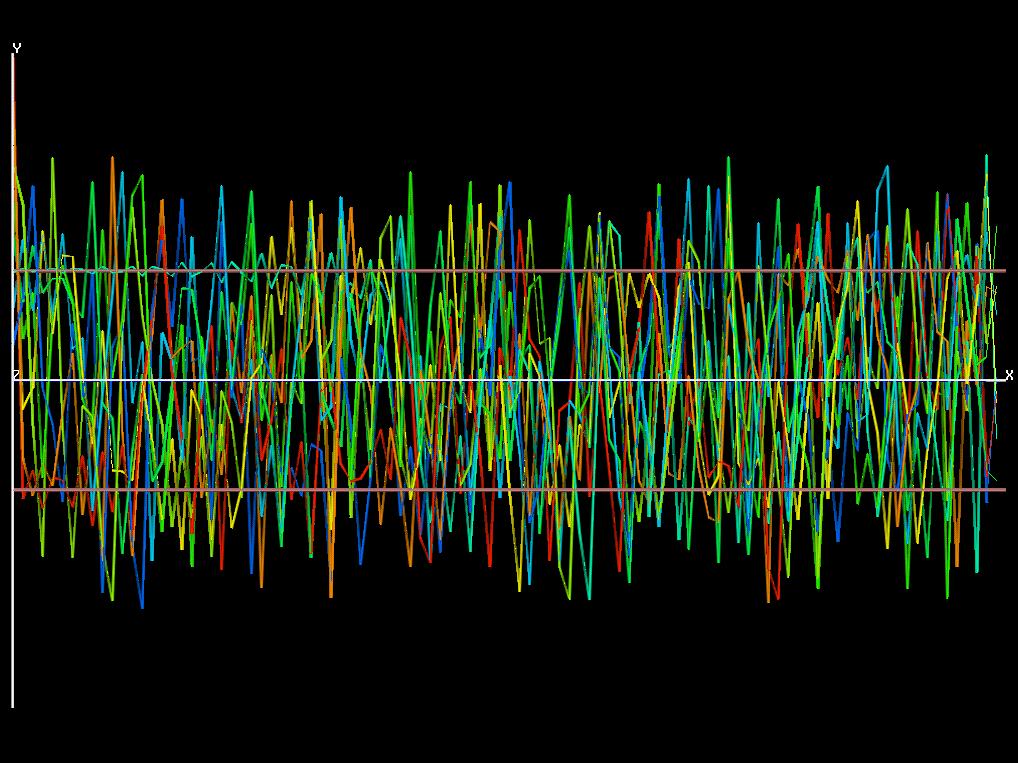
At r=24.74 the fixed points C+ and C- loose their stability by absorbing the
unstable limit cycle (see dashed line in the above bifurcation diagramm)
in a supcritical hopf bifurcation.
The waterwheel changes rotation speed and direction erratically.
Left image (143K): r=28.0, 10000 iteration steps, 10 starting points |
|
When decreasing r the unstable limit cycles expand until they touch at
r=13.962. Below 13.962 there are no limit cycles (see image for r=6.0 above).
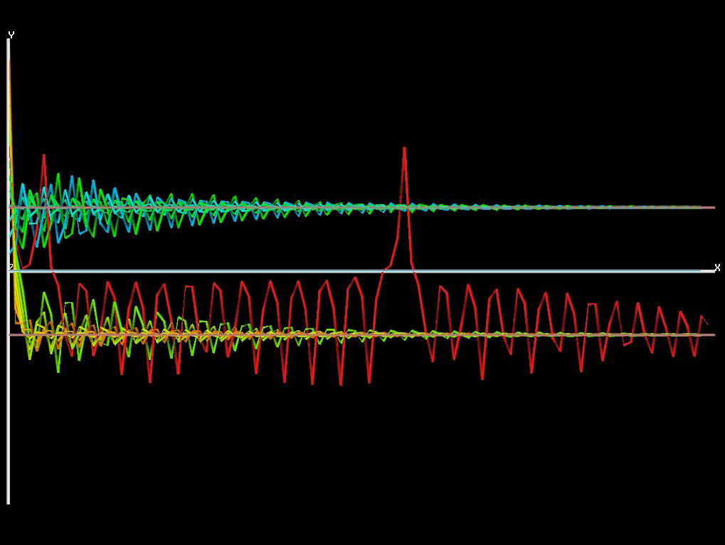
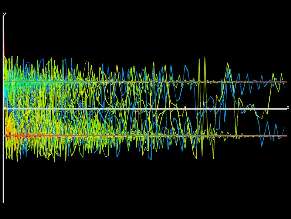
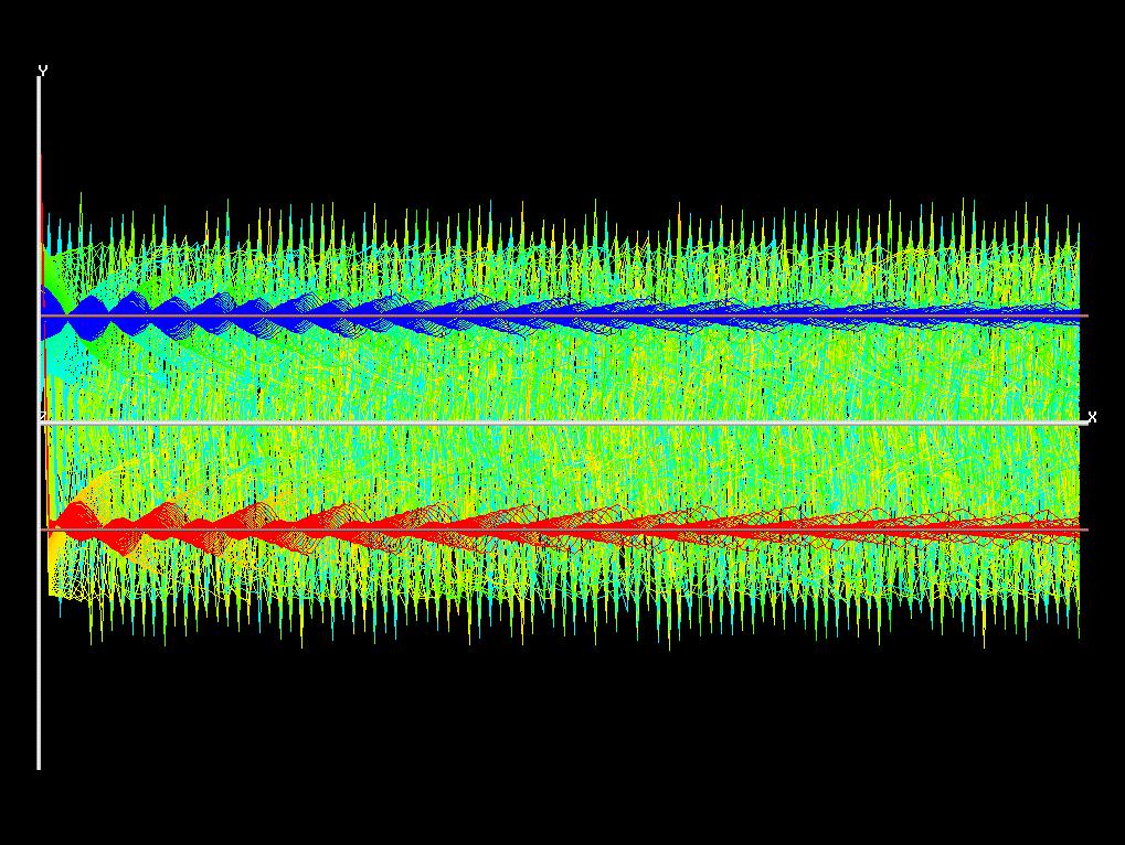
Between r=13.926 and r=24.06 the Lorenz system exibits transient chaos.
Trajectories can rattle around chaotically for some time. Eventually they
settle down to on of the fixed points C+ or C-.
Left upper image (64K): transient chaos for r=19; red colored trajectory: the waterwheel changes its direction after several turns and immediately changes it again before the rotation tends to become steady. Left middle image (128k): transient chaos for r=21 many trajectories change their sides, i.e. the waterwheel changes it direction. After 10000 iteration steps most trajectories have reached one of the fixed points C+ or C-. For the waterwheel it means that most initial conditions have settled in a steady rotation. Left lower image (96K): r=19.0, transient chaos, the trajectory changes its sign in x (and y) twice before it approaches a stable fixed point. Time is color-coded. |
|
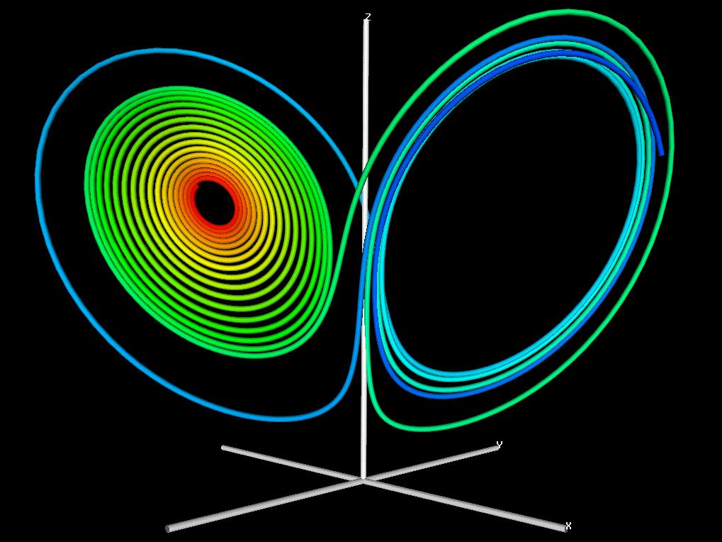
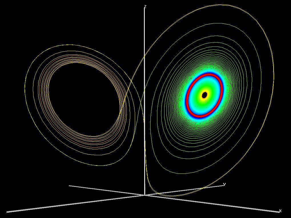
Above r=24.06 the system is a strange attractor.
A trajectory being outside the limit cycle is not able to enter it after
any time as it was the case for transient chaos. Only trajectories starting
within the unstable limit cycle or on specific points, that are not on
the attractor, reach a fixed point, i.e. steady rotation. Upper image (209K): r=24.1 Only the trajectories that start at a point near a fixed point C+ or C- reach the fixed point. Here also some trajectories starting at a point that is not on the attractor reach the limit cycle. These trajectories are colored blue and red. All other trajectories exibit chaos and are color-coded in dependence of thei initial condition as described above. Lower image (122K): The red tube shows the limit cycle for r=24.1. Trajectories starting inside the limit cycle reach the fixed point C+. Trajectories starting outside the limit cycle move away from it never getting inside a limit cycle of C+ or C-. Two trjectories are visualized. One is starting inside the limit cycle, the other trajectory starts outside the limit cycle. Time is color-coded. Both trajectories start with blue color and end with yellow color. |
Two animations (MPEG) have been made to illustrate to long time behaviour while varying the parameter r.
| r is varying between 0.5 and 1.5 to illustrate the changes in stability at r=1. |
| In this animation r is varying between 0.0 and 26; from "one attracting fixed point" to "strange attractor". |