"Lowest-Variance Streamlines for Filtering of 3D Ultrasound" implementation

Julian Wagner

Downloads

• Executable
• Source
• Doxygen Documentation

Description

This application is a implementation of the paper "Lowest-Variance Streamlines for Filtering of 3D Ultrasound" from Veronika Šoltészová, Linn Emilie Sćvil Helljesen, Wolfgang Wein, Odd Helge Gilja and Ivan Viola.

It is an approach to reduce speckle noise in 3D ultrasound images. The difference regarding other filters is, that the filter kernel is computed with a process, similar to streamline integration. This is, e.g., done to gain better results on bordering tissues. In the first step, the variance for every voxel in different directions is calculated. The direction with the lowest variance is then written in a 3D vector field, to the position corresponding to the voxel.

In a second step, we sample along the streamlines in our 3D vector field and calculate the arithmetic mean of the corresponding voxels in our volume.

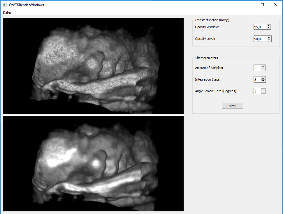
For comparison and comfort, I wrapped the algorithm in a rudimentary volume renderer using VTK and QT.

Guide

A Nvidia GPU with CUDA capabilities is needed to execute the program. After execution, you can load a volume (META-Image format) in the upper left corner. You can rotate, translate and zoom the rendered volume in the upper window. You can also adjust the transfer function to your likings. Before you start the filter process, you can change a few parameters.

• "Amount of Samples" lets you choose how many samples you want the algorithm to compute during the variance computation (in each direction).
• "Integration Steps" lets you choose how many samples you want the algorithm to compute during the streamline integration (in each direction).
• "Angle Sample Rate" lets you choose how many degrees are between each sampled direction.

How to build

The volume render part of the project comes with a CMake file. As the filter part is developed using CUDA, it has to be compiled with the NVCC compiler. I would recommend to build it as a static library and to link it against the volume renderer.

Implementation

Filter

The filter is programmed in nvidia CUDA and consists of two steps, that execute sequential on the GPU. If the amount of voxels does not exceed the amount of parallel threads on the used GPU, all voxels are computed parallel and individually.

In the first step, each thread samples the variance along every given direction for one voxel. The direction with the lowest variance is saved in a vector field. This step is the computational most expensive one. Therefore optimization was in order. E.g., switching from a naive two-pass approach for calculation of variances, to a single-pass approach yielded 2 seconds of computation time.

The second step consists in sampling the volume along the calculated streamlines. For this part the authors of the paper use a Runge-Kutta-4 like scheme, which I also implemented.

Volume Renderer

The GUI for the volume renderer is built using QT 5.8, in addition with widgets from the VTK. For rendering I utilised the vtkSmartVolumeMapper.

Libraries

• VTK -7.1.1 for the volume renderer.
• nvidia CUDA for the parallell execution of the filter kernel.
• QT 5.8 for the user interface.

Performance

The results of nvprof for a volume with 273x151x193 voxels can be seen here:

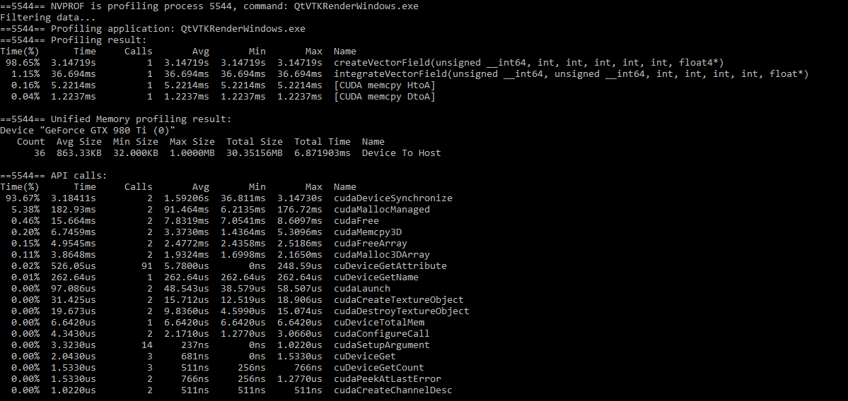
• "Amount of Samples" 5
• "Integration Steps" 5
• "Angle Sample Rate" 5