
Kinetic Visualization is an approach, which tries to utilize animations (the motion of particles) to
enhance the perception of the shape and texture of a static object.
The idea originates from observations that e.g. an object in moving water gives the perception of a shape. The modeling method for kinetic visualization is based
on a particle system using (physical or biological) rules to update each particle, define interaction between particles
and render the particles. The proposed technique is not a replacement for conventional rendering methods e.g. direct volume rendering.
Features
- Coherent Movement (Flocking/User Preferred Direction)
- Collision Avoidance (Repulsion/Dying)
- Gaussian Filtered Image
- Particle Shading
- Transferfunction Manipulation
- Configuration File
Technologies
Requirements
- Windows XP, Vista, or Windows 7 machine
- OpenGL-compatible graphics card and OpenGL 3.2 (or later, CUDA is recommended)
Test Environment
- Desktop-PC: Windows 7 64-bit; Intel Xeon 3GHz; 4 GB RAM; Nvidia Geforce 9600 -> 115 fps (Nucleon)
- Notebook (Thinkpad T61p): Windows 7 32-bit; Intel Core 2 Duo T7800 2,6 GHz; 2 GB RAM; Nvidia Quadro FX 570M (256MB) -> 38 fps (Nucleon)
Runtime Settings
The runtime configuration settings are for all configurations, which are used for manipulating the motion strategies of the particles (as described in
chaper 3).

General Movement (chapter 3.2)
- Stick Particles to Density Level: Precomputation of a position and change it, if the position does not fit on the volume.
- Curvature Influence: Defines how much the principal curvature direction influences the particle direction (variable kc in the paper).
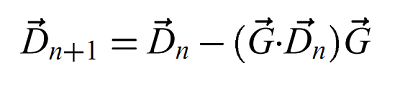
Note that the following formula of the paper (chapter 3.1 - Motion Along the Surfaces) is always used and is independent from the user parameters:
Coherent Movement (chapter 3.3)
The parameter settings for flocking and user preferred direction are responsible that the particles move in directions consistent with their neighbors.
Flocking
Flocking is implemented by weighting the direction vectors of a particles neighbors with a gaussian. Sigma indicates the size of the gaussian and Flocking influence is described in the paper.
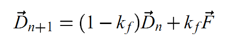
- Flocking Influence: Defines how much the flocking is influencing the principal curvature direction (variable kf in the paper).
- Flocking Sigma: The sigma for calculating the flocking vector (variable F in the paper) according to Multivariate Normal Distribution.
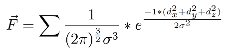
The sigma sign means in this context, that this calculation must be done for every neighbor of a particle (there is an iterator ParticleMapIterator implemented for getting the neighbors).
User Preferred Direction
The alternative to flocking is to simply define a user preferred direction for the particle movement.
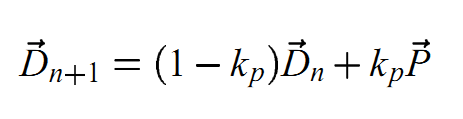
- User Direction Influence: Defines how much the user direction is influencing the principal curvature direction (variable kp in the paper).
- User Direction X, Y, Z: The actual direction (variable P in the paper).
Collision Avoidance (chapter 3.4)
In order to get a well distributed particle density, the application provides magnetic repulsion and particle dying.
Repulsion
The repulsion radius indicates how big the neighborhood should be, which should be checked. Repulsion influence is described in the paper. Particles will be moving away from
each other inverse proportional to the square of their distance (also desribed in the paper in chapter 3.4). This approach is quite similar to
Newton's law of universal gravitation or
Coulomb's law, because here is also the inverse square of the distance the basis of most calculations.
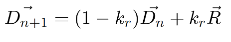
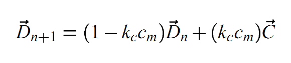
- Repulsion Influence: Defines how much the repulsion vector influences the previous calculated direction of the particle (variable kr in the formula).
- Repulsion Radius: Used for calculating the repulsion vector (R in the formula).
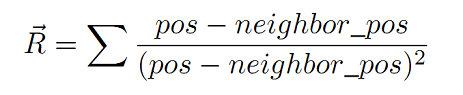
As for the flocking vector, the sigma sign means in this context, that this calculation must be done for every neighbor of a particle.
Dying
Particle dying is implemented by counting each neighbor and weightening it with a gaussian. If this sum is above the threshold the particle will die.
- Crowdeness Threshold: If the sum of the gaussian from all particle neighbors is above this value, then the particle dies.
- Crowdeness Sigma: The value, with which the gaussian for getting the neighbors is used.
Preprocessing Settings
The preprocessing configuration settings are for all initialization steps of the particle system, which are also manipulating the motion of the particles and need to be done before
the actual rendering of the particle take place, such as motion along the surface (chapter 3.1), particle density (chapter 3.4), number of particles and so on. With this parameters
the particle system is generated in a loop (xyz - direction) in the class ParticleFactory.

- Preprocessing Gaussian Sigma: The volume is in the first step convolved with a gaussian in order to remove noise. Preprocessing Gaussian Sigma is the sigma parameter of
this gaussian. If Enable Gaussian Filter is off, then the particle system (size, density level, etc.) is generated on basis of the original volume image file.
- Density Level: Indicates the depth-level on which the particles are generated. Particles are only created if the depth level on the volume is ok.
- Density (inverse): Indicates the density with which the particles are generated. This parameter is used for determining if there is a free position for a particle, otherwise
the generation of the particle is aborted. If the density is big, the particle-field is initialized sparser. This parameter is also used in the runtime settings for the dying.
- Maximum Number of Particles: Self explanatory.
- Gradient Magnitude Threshold: Threshold which the dot(gradient, gradient) must exceed for particle generation on this position.
Rendering Settings
With the rendering settings, the user is allowed to change the parameters of the direct volume rendering technique and some other parameters of the particles, which are not
directly concerned with the particle system itself (e.g. particle size and particle shading).

- Sample Step: The step size which is added to the ray direction for determining the next ray position in the ray casting loop. The smaller the number, the better (and slower)
the rendering will be.
- Shading Intensity: Self explanatory.
- Gradient-Magnitude Shading Modulation: Determines how much the gradient magnitude influences the shading. This helps to decrease shading artifacts in homogenous regions.
- Gradient-Magnitude Opacity Modulation: Determines how much the gradient magnitude influences the opacity (alpha). This will enhance the visibility of interfaces between two regions.
- Particle Size: The size of the rendered particles.
- Render Gaussian Filtered Image: Take the gaussian filtered volume image (previously used for preprocessing stuff) for the direct volume rendering process as well.
- Particles Enabled: Turn on/off particle rendering in the raycasting fragment shader.
- Particle Shading Enabled: Turn on/off particle shading in the particle fragment shader.
Save Configuration Settings
It is possible to store all mentioned configuration settings in an ini-file.

Open Volume
Tha application can load dat- and dds-files. By selecting multiple image files, it is possible to load respectively build a volume.

The application works with all 8-bit volumes from The Volume Library. The 16-bit
volumes are not supported.
Preprocessing (CUDA and alternatively CPU)
In the preprocessing/initialization step, the application computes the gradient and the curvature of the volume image. Additionally in this step also the
gaussian smooth image is calculated.
The input for the preprocessing step is for example (Nucleon) the following image:

The class ProcessingUtils and ProcessingUtilsCuda computes now the gradient, curvature and gaussian smooth image of this input. If CUDA is not available on the target architecture, then this
computation takes place on the CPU, otherwise on the GPU with CUDA.
Gradient computation
The gradient is calculated like in GPU gems with central differences.
Curvature computation
The curvature is calculated according to Computing the Differential Characteristics of Isointensity Surfaces.
First of all the gradient for the image is calculated, which is the first derivation. After this the "gradient of the gradient" in x-,y- and z-direction is calculated for
the curvature computation, which is the second derivation.
Then a loop through the volume in each direction computes the curvature as follow (computes the principal curvatures from the first and second deviations of the image):
- The curvature computation for the 2D case:
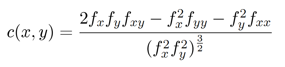
- The curvature computation for the 3D case (used for the implementation of the particle system):
- Compute K:
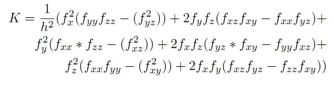
- Compute H:
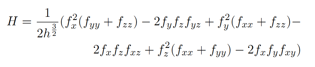
After this step alphaX, alphaY and alphaZ is calculated. With this results the ti's are calculated as follow:
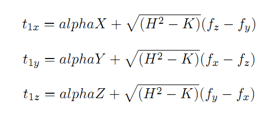
The ti's are then the curvature C = vec3(t1x, t1y, t1z). Please take a look at the paper for more details.
Gaussian computation
The gaussian computation is used for smoothing the image (remove some noise). This smoothed image is the basis for the curvature computation. It can be also used for rendering a
gaussian filtered image of the volume.
On the right side is the gaussian filtered image and on the left side is the non-filtered image.

Particle System
The generation of the particle system is located in the class ParticleFactory, while the rules for the particle system are implemented in the class Particle. Most of the steps are already
described in the user interface part of this documentation, but here a short overview:
- Calculate curvature, gradient and gaussian of the volume in ProcessingUtils.
- Generate particles once in ParticleFactory and take parameters like maximum particles, density level, neighbor radius etc. into account.
- Prepare step: Apply the rules of the particle system to the direction of each particle at each frame
- Update particle direction along curvature.
- Apply flocking or user preferred direction rules
- Do magnetic repulsion if enabled.
- Always apply the gradient rule which is independent from the parameters.
- Stick particles on the volume if enabled.
- Do dying if enabled.
- Apply the computations of the prepare step (direction) to the position of the particle and set the direction for the next iteration (each frame)
Two render passes
In the first pass the particles are rendered to an offscreen framebuffer. The particles are in the intervall [0,width] x [0,height] x [0,depth] and must be transformed to the cube
coordinate system [-10,10] x [-10,10] x [-10,10] of the volume. The depth texture is then passed to the volume fragment shader where the rendering of the volume and the visibility computation
of the particles take place.
Geometry Shader
The geometry for the particles is generated in the geometry shader particles.geo and is a simple rectangle (with the particle size as parameter). In the fragment shader particles.frag
of the particles a texture is used for obtaining nice particles.

Direct Volume Rendering
The application uses direct volume rendering (front-to-back compositing) with a transfer function.
Volume Shading
The volume shading is located in the fragement shader kinetic_particles_dvr.frag. We are using the blinn-phong light model for volume shading and as desribed
in we additionally do gradient magnitude shading and gradient magnitude opacity modulation. For shading we are
using one light source and the intensitiy of the shading can be manipulated by the user. Shading is performed in every iteration of the ray casting loop and thus has a great performance
impact (125fps vs. 75fps).
On the right side is the shaded volume and on the left side is the unshaded volume.

Particle Shading
The particle shading is located in the fragement shader particles.frag. Similarly to the shading of the volume, we use the blinn-phong light model for particle shading.


