Graphical user interface

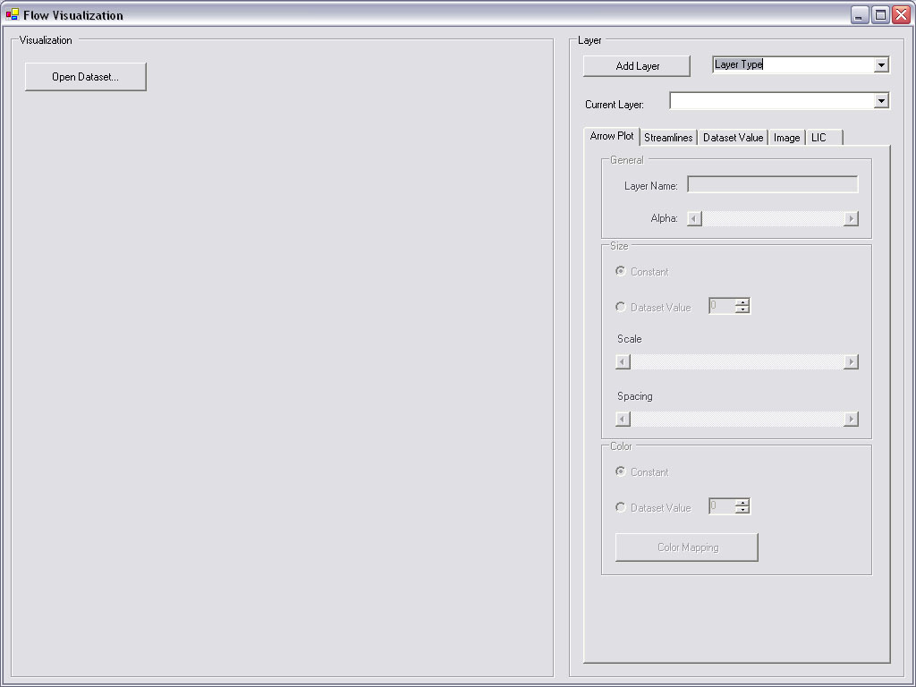
The main interface of the program looks like this:



Choosing "Open Dataset" opens up a file dialog which allows the user to load a grid file and a flow data set. After choosing an appropriate file, the user can start to build layers from the interface on the right.

Dataset Value Layer



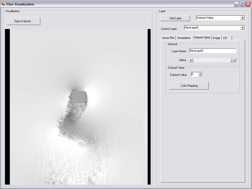
On the right-hand side, the layer can be named and an alpha value can be assigned to each layer, which allows several layers to be displayed on top of each other using alpha blending.
Furthermore you can choose which dataset value you want to see. By clicking on "Color Mapping", the user can define a custom color mapping in the dialog which looks the following:

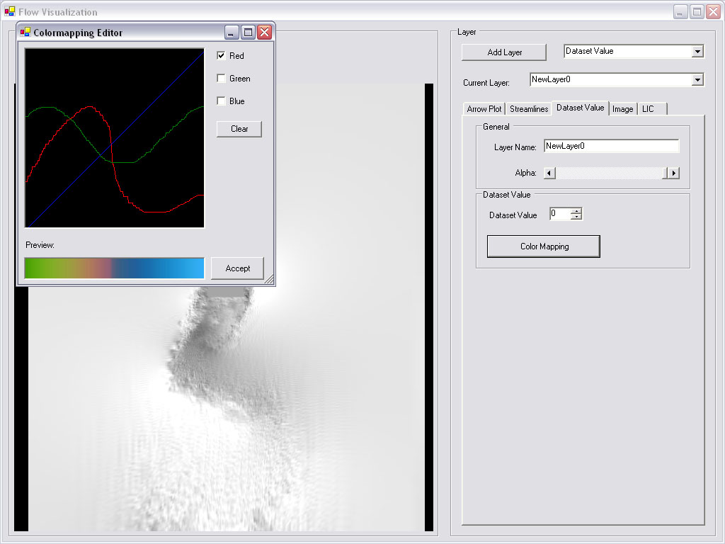
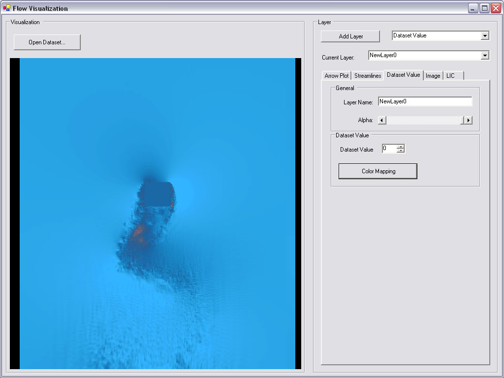
After drawing the color mapping function into the panel and clicking "Accept", the image gets immediately updated:

Arrow Plot Layer

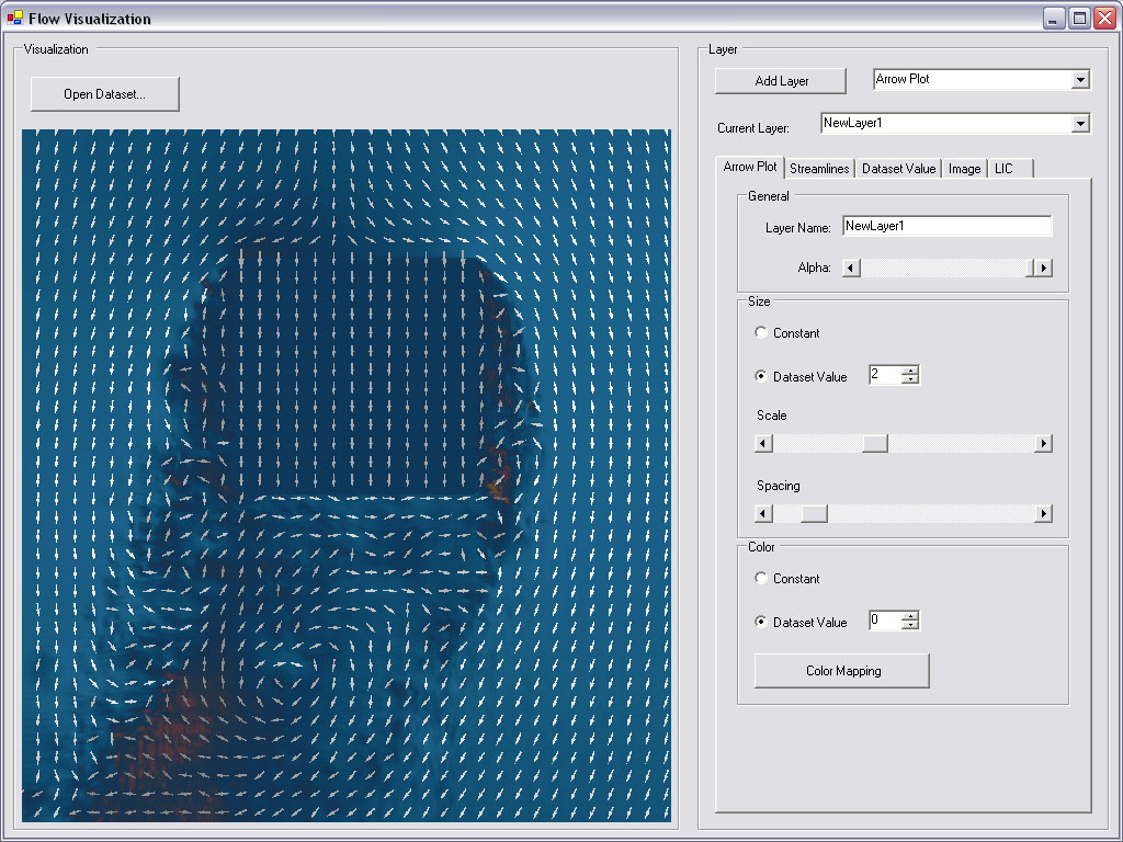
For the arrow plot layer, the user can choose between constant size or the size being dependent on a specific dataset value. Scaling and spacing between arrows can be changed using the two respective sliders. Like the size, the color can be constant or based on a dataset value with an additional color mapping.

Streamlines Layer

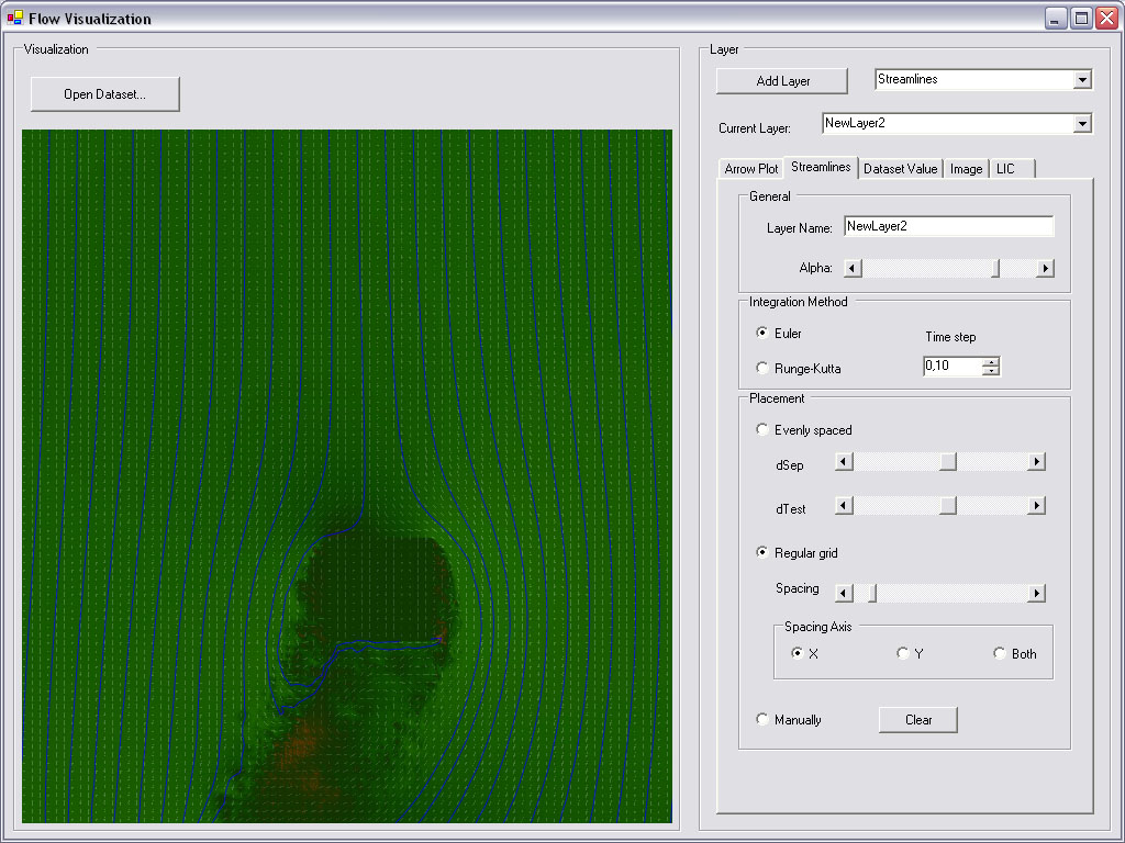
On the streamline layer there are several more options: The user can choose between two integration methods (Euler and Runge-Kutta) and set an appropriate time step. The placement of the streamlines can either be evenly spaced, based on a regular grid, or manually.

Line Integral Convolution Layer

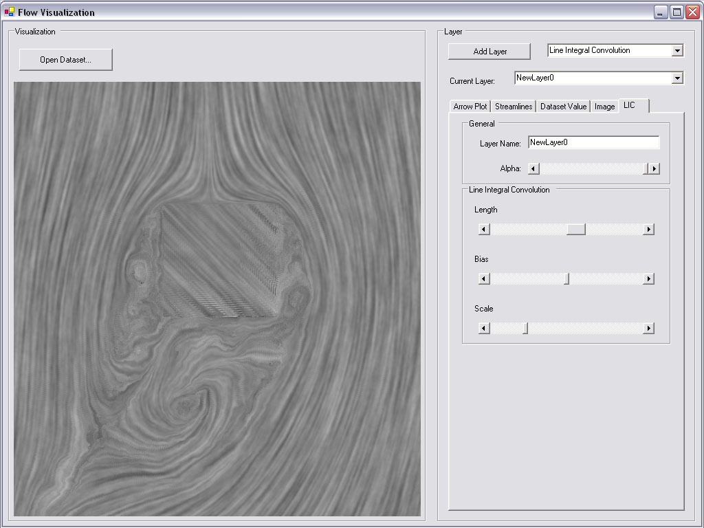
On the LIC layer the user can choose the length of the convolution - the longer the convolution, the more samples are taken in the GLSL-shader. Hence, the rendering will be slower. Using the bias slider it is possible to visualize the flow of velocity. The texture-offsets taken in the GLSL-shader also depend on the scale-slider which can be used to make the flow more or less visible.