Volume Rendering
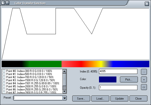
Direct volume rendering is the second visualization option. This uses raycasting to create an image from the input data set. Options include a variable viewport, various combination strategies and a freely defineable transfer function for converting sample values to color and opacity values.

Renderer selection
Volume rendering is activated by selecting the "Ray-Casting" radio button inside the group box entitled "Rendering methods". Additional options have interfaces of their own that can be shown using the three buttons "Show camera control", "Show raycasting options" and "Edit transfer function".


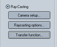
The raycasting option selected

Camera setup
This option comprises a full setup for an origin-centric viewport in R3. This means that the data set is always interpreted as being centered at the origin of karthesian space with the camera being located a certain distance from it and rotated a certain amount around each of the principal axis.



Distance
Distance is given as a factor of the longest extension of the data set. This means that if the data set has dimensions of 512x512x256 then the distance of the eyepoint from the origin can range from 2.0 * 512 to 8.0 * 512. We have found that a start factor of 2.0 guarantees full visibility of the data set. Higher factors allow for smaller screen areas to be filled which directly corresponds with faster rendering times.

Rotation
Rotation is given in degrees around each of the principal axis. Viewport construction works by initializing a position at the origin (0/0/0) with a view vector down z-axis (0,0,-1). This is translated away from the origin along the z-axis and the rotated first around the x-axis, then around the y-axis and finally around the z-axis.

Rendering options
Raycaster rendering has four principal options - combination strategy, threshold value, ceiling value and type of interpolation.



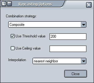
The "Use Threshold value" and "Use Ceiling value" options allow to limit the scope of sample values taken into account during value extraction. Both are specified in a range of [0..4095] in accordance with the 12 bit value range.

Combination Strategy
The combination strategy defines how values that are extracted from the data set are combined into the final sample value. Current options include as follows:

• First hit - Samples are collected along the ray until the first sample value above a certain threshold is found. The threshold is either 0 or the threshold value available as an option.
• Average - Samples are collected along the ray while it pierces the data set. All sample values are summed up and then divided by the number of samples found. The final value determined is the average of all values found.
• Maximum Intensity Projection (MIP) - Samples are collected along the ray while it pierces the data set. Of all samples found, the highest sample value is used as final value.
• Compositing - Samples are collected along the ray while it pierces the data set. Sample values are composited according to the current transfer function.
  

Interpolation
Interpolation determines how sample values taken are extrapolated from the data set. Options include nearest neighbor interpolation where the value from the closest cell is used and trilinear interpolation which combines the values of all 8 neighboring cells according to their distance from the actual sample position.

Transfer functions
The current transfer function can be edited in a seperate window which looks like this:



Opacity graph and color gradient
The graph at the top shows the development of the opacity from minimum to maximum sample value. Right below is the color bar that shows the color gradient over the sample space.

Point List
Below the graph and gradient there's the point editing area. On the left is the list with all points listing for each point index number, sample value index, RGB color value and associated opacity.

Command Buttons
"Save" and "Load" buttons (will) allow to load and save a transfer function from and to a text file. This function is not yet complete. Clicking "Update" redraws the opacity graph and color gradient. "Close" will do just that.

Optimizations

Examples



Example 1: A CT scan of a christmas tree. Threshold is at 200, Ceiling value at 2000. Transfer function takes gradient from full black to full white in [0,2000]. First hit combination strategy is used.




Example 2: The same view of the same tree, using Average as combination strategy.




Example 3: Same, as above. Maximum Intensity Projection used as combination strategy.