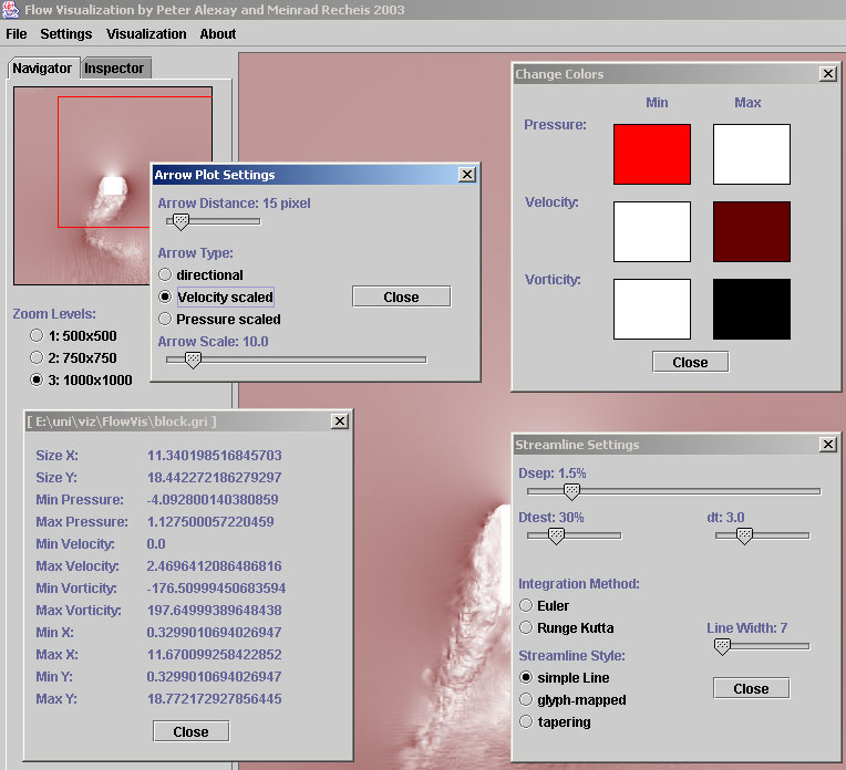
FlowVis in action. You can see in this picture the navigator tab and the viewport in the background, and all the dialogs in the front.
by Peter Alexay and Meinrad Recheis
done for the Visualization Course at the Institute for CG - TU Vienna
Flow Visualization of a computer simulated dataset of directional velocity, pressure and vorticity at points in 2-Space. The Program was written in Java and Python and needs Jython installed. Most of the visualization algorithms were coded in Java due to performance reasons. The GUI was scripted in Python using the javax.swing package, because Python has more power and a less complicated syntax/language design. (see the source doc for more information).
To build the program from source you must first comile the *.java files with specifying the classpath of the jython package like this: javac -classpath ./jython.jar *.java
(the jython.jar comes with the jython distribution)
Then run the python script FlowVis.py by typing jython FlowVis.py in the command promt.
The source code may be redistributed or changed under the terms of the GNU GPL, that is: any program derived from this program must be declared as open source under the GNU General Public Licence.
download: source.
a brief source documentation
the jython.jar that is needed to compile the java source
the data set: gridfile, datafile. Note: there are two similar versions of this files that differ in their endianness. our program is able to load only the linked ones. The data files have their own license including a description of the data format.
the jython installer (java-class).
The program is able to load a grid-file and the linked data-file and provides some methods to visualize the flow of a liquid that is blocked by a barrier.
Featured Visualization Methods:
* Color coding of velocity, pressure and vorticity
* Two different arrow styles
* Simple Streamlines and Evenly Spaced Streamlines
* Three different streamline styles
User Interaction Features:
* Zoom
* Data inspection per mouse
* Interactive customization of the visualization tools
Coding Technology: Interfacing Java and Python
* Low level algorithmic code glued together by a high level script language
|
FlowVis in action. You can see in this picture the navigator tab and the viewport in the background, and all the dialogs in the front. |
| Click to see the original size screenshot |
 |
 |
|
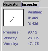
| The inspector shows the data values at the mouse cursor (in percent of the range [min..max]) and a velocity scaled pin arrow, to visualize the direction of the flow. | ||
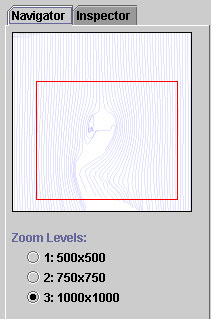
| The navigator shows the current view and allows to switch between three zoom levels, which are given by the pixel size of the canvas. | ||
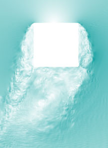
Background Color Coding:
 |
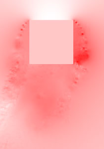 |
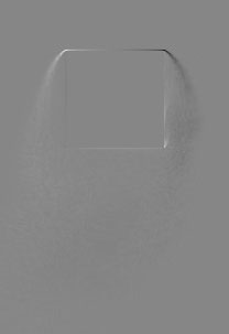 |
| Velocity | Pressure | Vorticity |
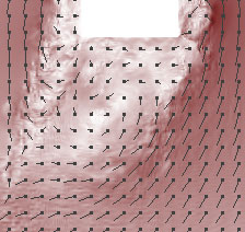
Arrow Plot:
The arrow plot is a relatively simple tool for visualizing flow direction.
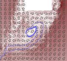 |
 |
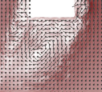 |
| Simple directional arrows | Pin glyph scaled by velocitiy | Pin glyph scaled by pressure |
|
Background: velocity |
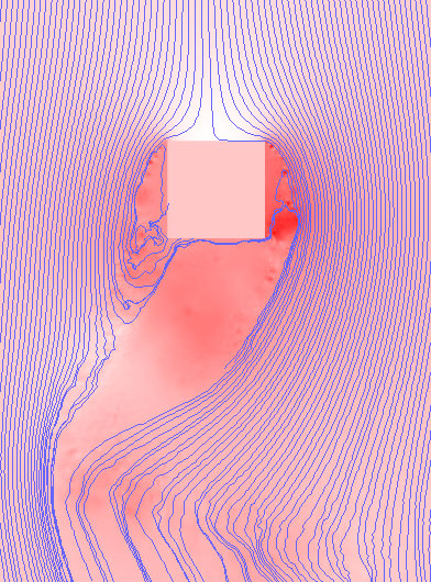
Simple Streamlines:
The idea of streamlines is based on the concept of injecting colored particles into a flow to visualize the change of the medium over time as it passes a solid body.
The visualization with simple streamlines has two disadvantages: on the one hand the streamlines do not cover large parts of the flow field, like the vortices, on the other hand they are sometimes too dense.
Comparison of two integration methods for streamlines, see [2].
 |
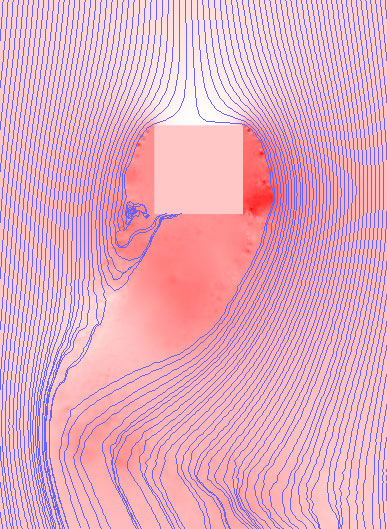 |
| Euler Integration | Runge-Kutta |
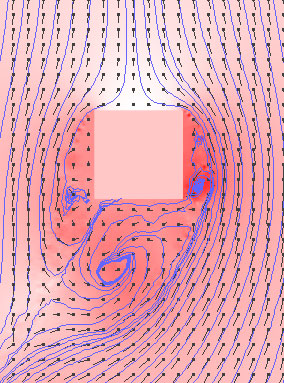
It seems that the streamline visualization is quite more expressive than the arrow plot approach, but streamlines lack of directional information. It is either possible to print the two methods over each other or to combine the advantages of both methods which results in glyph mapped streamlines. we use a tear drop glyph to visualize the flowing direction.
 |
 |
| User placed streamlines with velocity pins | User placed glyph mapped streamlines |
Evenly Spaced Streamlines (ESS):
This algorithm detects when the gap between two streamline is too large and inserts new streamlines or removes streamlines if the distance between them is too small.
Two screenshots with different integration steps, that means different accuracy. the computing time can be very long with a small step.
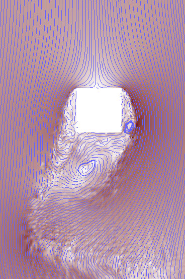 |
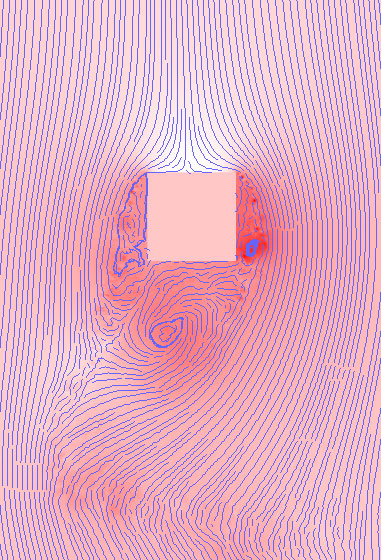 |
|
| integration step dt: 3.0 | integration step dt: 2.0 (more accurate) | |
| both Euler, Dsep: 0.5, Dtest: 70 |
[1] "Vector Algorithms", chapter 6.3 in William Schroeder, Ken Martin, Bill Lorensen, "The Visualization Toolkit", pp. 155 - 162, Prentice Hall, 1996
[2] Bruno Jobard and Wilfrid Lefer, "Creating Evenly Spaced Streamlines of Arbitrary Density", Visualization in Scientific Computing '97, Springer Vienna, 1997, pp. 43 - 54
24.02.2003 Meinrad Recheis