Within the scope of the LU Visualisierung we implemented a ray-casting  algorithm. This  means that an image is generated without any geometric primitives, for every pixel a ray is casted through the volume data to obtain the color and transparency information on that location.

The task was ..

1) .. to display slices in the x-, y- and z-axis

2) .. to easily change the the color mapping of density values in the volume data

3) .. to provide different volume rendering modes

4) .. to be able to arbitrarily rotate the volume data and the light source

- Slice Rendering (nearest-neighbour and bilinear data interpolation)

- Average Density Rendering (x-ray style) (nearest-neighbour and bilinear data interpolation)

- First Hit Volume Rendering

- Volume Rendering with accumulated color intensities

- Threshold Rendering in both modes

- interactive color mapping control

- interactive volume and light positioning control

By default the slices are rendered using nearest-neighbour interpolation, which means in our case that every pixel on the screen is associated with one voxel in the appropriate slice. Therefore the program provides image interpolation methods (voxels only, nearest-neighbour, bilinear and bicubic), which comes into account when the user resizes the image. Then those pixels that not directly map to a voxel are interpolated according to the selected method.

On the other hand we can select bilinear data interpolation, which interpolates the density values for the neighbouring voxels linearly.

Slice Rendering

using nearest-neighbour image interpolation

Slice Rendering

using bilinear data interpolation

The program provides an easy way to edit the mapping from density values in the volume data and the color and transparency values on the screen.

It is also possible to load and store the current state of the transfer function to ease the handling.

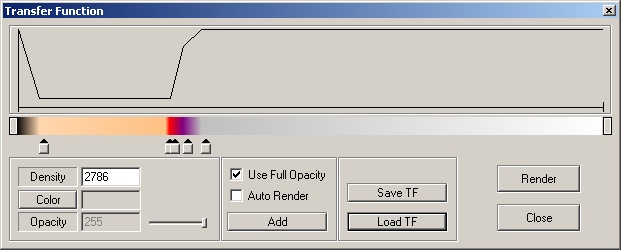
Transfer Function

with a loaded color mapping

This is only a little add-on ..

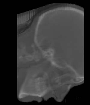
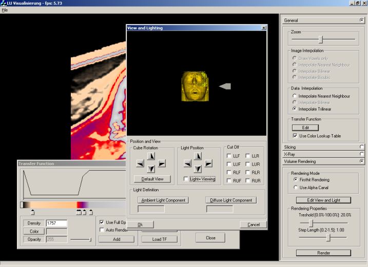
X-Ray Rendering

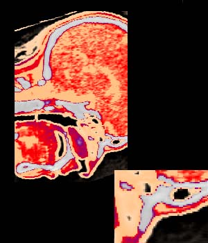
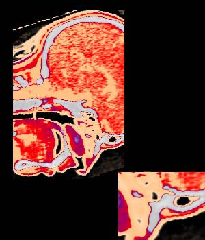
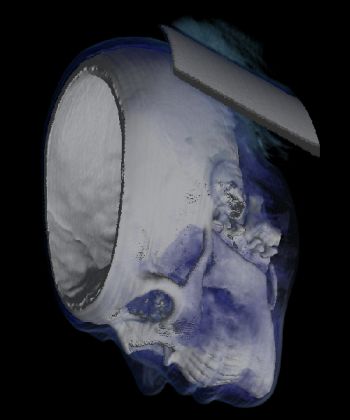
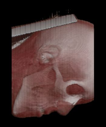
Generally here the user has two methods to choose from: first-hit rendering (Figure A+B) or accumulated color rendering (Figure C+D). Moreover it is a threshold slider provided to cut away certain portions of the volume data (Figure E+F). In addition we can cut away parts not defined by the density value, but defined by the location of the part (Figure D+F).

There is some more we can see here: different transfer functions and different light settings.

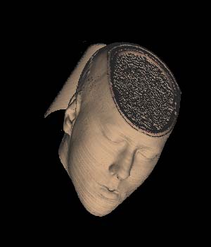
Figure A

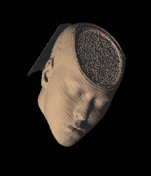
Figure B

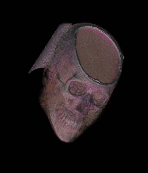
Figure C

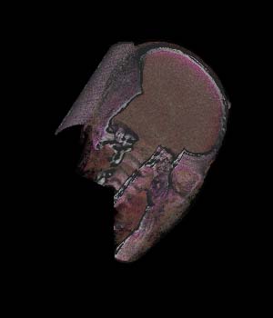
Figure D

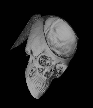
Figure E

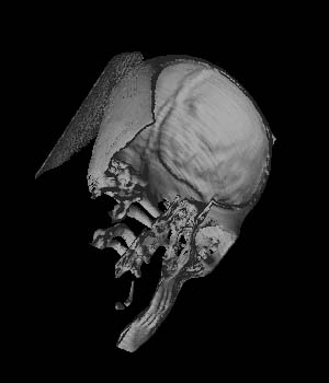
Figure F

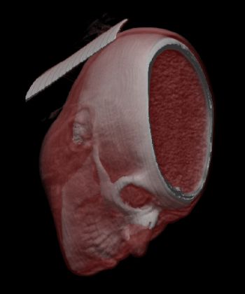
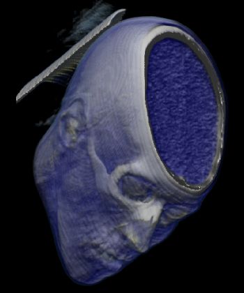
Some better screenshots ..

Volume Rendering

grey light, blue + alpha <1% for skin densities (~250)

Volume Rendering

grey light, red + alpha ~15% for skin densities (~250)

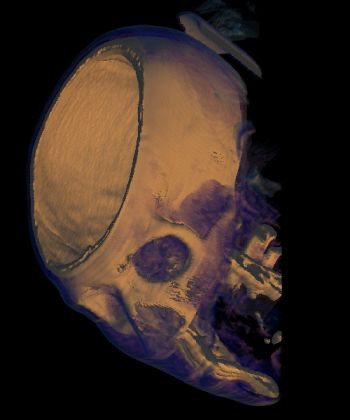
Volume Rendering

orange light, blue + alpha ~1% for skin densities (~250)

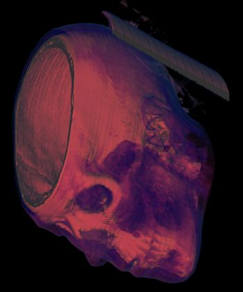
Volume Rendering

red light, blue + alpha ~1% for skin densities (~250)

Volume Rendering

grey light, red + alpha ~15% for skin densities (~250)

Volume Rendering

grey light, blue + alpha ~15% for skin densities (~250)