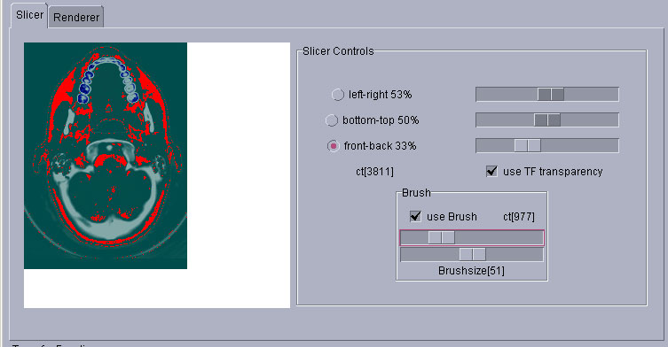
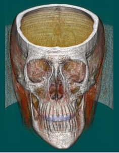
Slicer in action: The bones are colored white and even higher densities are colored blue (teeth). Less dense tissue is transparent, the background is green. Tissue densities +-25 around 977ct are colored red by the brush.
by Peter Alexay and Meinrad Recheis
done for the Visualization Course at the Institute for CG - TU Vienna
Volume Visualization of a 3D dataset of densities acquired with computer tomography.
The Program was written in Java 1.3.1 and uses the package javax.vecmath. Run the program by typing java -Xms200M -Xmx256M VolvisMain in the command promt.
download: java source (kontaktiere die Übungsleitung) and java executables and the datafile.
a brief source documentation in German
The Program is able to load a CT-dataset and provides two major methods of visualization: "Slicing" and "Volume Rendering".
Slicer in action: The bones are colored white and even higher densities are colored blue (teeth). Less dense tissue is transparent, the background is green. Tissue densities +-25 around 977ct are colored red by the brush.
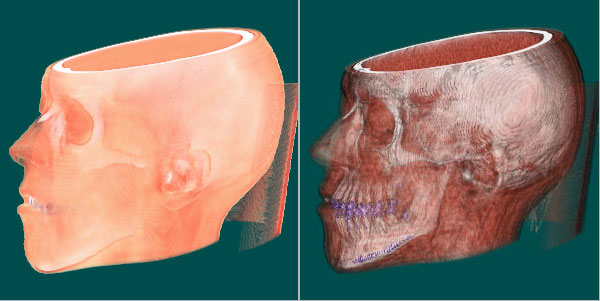
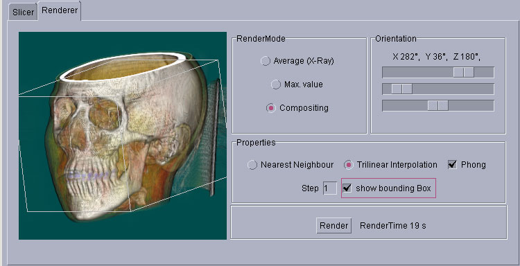
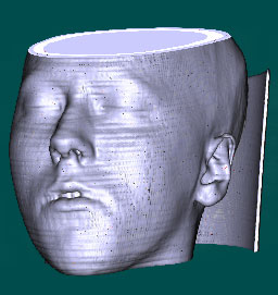
Renderer in action: Same transfer function as in the above screenshot. Uses gradients that is (vectors of change in density) for phong lighting. Because of the long rendertime (between 1 and 19s on a AMD 1800 XP for this volume data file) we added a bounding box (which can be hidden) to enable interactive orientation of the volume.
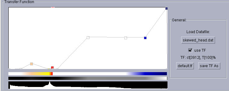
The transfer function used for both screenshots above: The two bars show the interpolation of colors and transparencies. The thing that looks like a landscape is the histogram of the dataset. We have taken the actual values to the 0.25th (that is the square root of the square root) to get it like this, otherwise it wouldn' t have been a usefull visualization of the distribution of the densities. On the left side of the histogram you can see an increase of densities which we set to fully transparent in our TF. Why? It is just noise.
[1] Marc Levoy, "Display of Surfaces from Volume Data", IEEE Computer Graphics and Applications, Vol. 8(3), pp. 29-37, Feb.1987
More Pictures:
above: different transferfunctions for the same volume data file with different orientation.
below: no gradients vs phong shading