VOLUME RENDERING -
RAYCASTING
by Thomas Lidy
This application is for the visualization of medical data, which was aquired from a CT-scan (computer tomograph). It allows you to select from a choice of different visualization methods, ranging from viewing slices of the human body to 3-dimensional Volume Rendering. The core algorithm used is Raycasting. The Volume Rendering algorithm is based on the scientific paper of Marc Levoy ("Display of Surfaces from Volume Data", IEEE Computer Graphics and Applications, Vol. 8(3), pp. 29-37, Feb.1987). You can find a summary of the Volume Rendering algorithm in German language here.
Installation:
requires:
- Windows
- ca. 162 MB RAM
- glut32.dll (included)
- comctl32.dll (should exist in C:\Windows\System)
- Data File: "skewed_head.dat"
Please unzip the files in a directory of your choice. Download the data file, unpack and save it to the same directory.
DOWNLOAD (kontaktiere die Übungsleitung)
Features
The application lets you select from 4 different kinds of visualizing the data set:
- Slices: to view a 2D slice inside the volume along an axis
- X-Ray: calculates average values through the data and shows a sort of an X-ray image
- Shading: normal shading of the data with light source to give a 3-dimensional impression
- Volume Rendering: enables you to view different tissue types at once by showing semi-transparent layers
The four features and their options are described in
detail below.
Every visualization method - except Slices - lets you
choose the view position by defining a rotation around
the X, Y, or Z-axis in degrees (-360 ... 0 ... 360).
Starting
Just run the file Raycasting.exe.
You will see 2 windows: The parameter window
and the drawing window.
 Immediately
upon startup, the data file is loaded, and the gradients
are calculated. You can see the calculation of the
gradients on the progress bar. At the
bottom of the parameter window there is the log
message box, which always informs you about what
currently is being done.
Immediately
upon startup, the data file is loaded, and the gradients
are calculated. You can see the calculation of the
gradients on the progress bar. At the
bottom of the parameter window there is the log
message box, which always informs you about what
currently is being done.
To get an image, select one of the four visualization methods (see below). After adjusting the desired parameters, click on the "Calculate + Draw" button. The calculation process is shown on the progress bar. (Sometimes, multiple calculation processes have to be done.)
The size of the output image is automatically adapted to the current size of the output window.*) Hint: You can also start the calculation/drawing process by a right mouse click in the output window, which is especially helpful if the size of your output window is so large that it covers the parameter window.
*) except with the Slice Viewer
Parameter
The only command line parameter Raycasting.exe accepts is a data file name as first parameter. If no data file name is given, the application automatically assumes "skewed_head.dat".
The data set
The data set from the CT-scan represents a 3-dimensional volume space, given a value for each voxel (volume element) which represents the density value of the human body at a certain position. In the data set, which was used while developing this application (skewed_head.dat), each voxel has a 12-bit value, so the density ranges from 0 to 4095.
The Slice Viewer and the X-Ray Visualization use these density values to calculate grey scale images, which enable you to distinguish between regions of different density.
For Shading and Volume Rendering, gradients are calculated from the density values, which are used for calculating normals for lighting and opacity calculations.
Raycasting
The technique behind the visualization methods in (2), (3) and (4) is Raycasting. This method is based on voxels - not on surfaces, like other rendering methods. For each pixel on the view plane, a ray is cast through the data set along the viewing direction. First, ray intersection points with the data volume are determined to identify rays, or ray parts, which lie outside the data set. Then colors (and opacites) at evenly spaced locations along the ray are computed (optionally by trilinear interpolation). According to method (2), (3) or (4) the colors and/or opacities are either summed and averaged, or multiplied together - either through front-to-back or back-to-front compositing - yielding a 2D image representation of the 3-dimensional data.
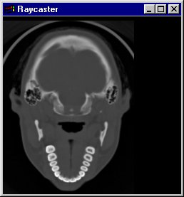
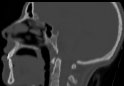
(1) Slices
The Slice Viewer allows you to view slices along one of the 3 axes as grey scale 2D images. Choose one of the 3 axes (X, Y, Z) and walk through the data along this axis with the Slider Control. The text box shows the number of the slice; the maximum is the x-, y- or z-Dimension of the data set, respectively.
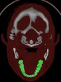
If you switch on the option "use colors (ranges)", the Slice Viewer shows the colors of the according ranges (Skin, Bones, Teeth - see (3)).
Note: The Slice Viewer automatically redraws the output image in the Rendering window while moving the slider.
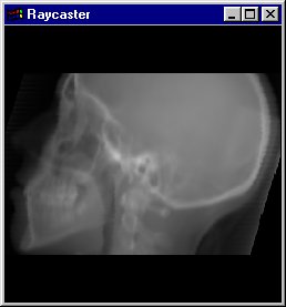
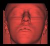
(2) X-Ray
The X-Ray viewer computes average density values along a ray, which is cast through the data and visualizes the density values as grey scale images, similar like the Slice Viewer does. However, you can rotate the view of the data set in any of the 3 directions, like you can do with Shading and Volume Rendering. Therefore, basically also the same raycasting algorithm is used as with Volume Rendering.
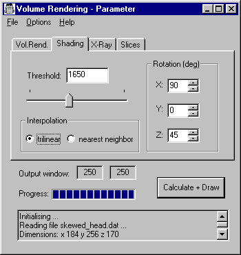
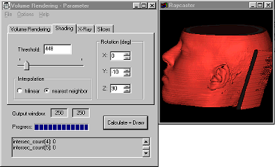
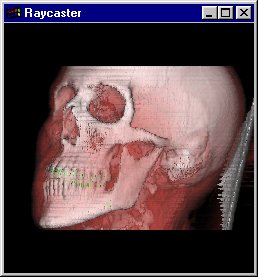
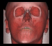
(3) Shading
When this rendering option is selected, a Shading model (Phong or Gouraud shading model) is used to calculate a 3D view of the data set. Normals are calculated from the gradients and a light vector is used to gain a "realistic" view of the data set.
The threshold value is used to select the density region, where the shading shall be applied. According to the values in the dataset, the threshold values range from 0 to 4095. You will get a visualization of the human's skin with values around 400, bones are shaded with values from 1700, and with a threshold of 3200, you will only see the teeth.
You can use the 3 rotation options to get an image from an arbitrary viewing position. The light vector moves with the view vector. You can choose between nearest neighbor interpolation and trilinear interpolation for calculating the shading colors (for an explanation of these options see (4)).
The shading model additionally uses highlights, when you switch on "Shading with Highlihts" in the Options Menu.
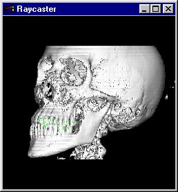
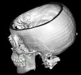
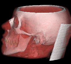
(4) Volume Rendering
Volume Rendering is the core feature of this
application. The disadvantage of normal shading with a
threshold is, that you can visualize only one tissue type
of the human body at once.
With Volume Rendering, each tissue type is assigned an
opacity; there are tissues, which are more transparent,
like the skin, and tissues, which are less transparent,
e.g. the bones.
For each voxel, a color which is basically gained from the same shading model as in (3) is computed. 3 ranges are defined in the application, which assign different colors and opacities to the skin, bone and teeth regions.
The (shaded) colors along the ray are multiplied by the voxel opacities, and composited in back-to-front order (see Raycasting). Note: The voxel opacities are directly influenced by the magnitude of the gradients of the data set.
As a result, you will get an image with differently colored tissue types, each having another transparency. The advantage of this method is, that you can recognize multiple tissue types of the human body in a single image.
You can set the desired viewing position with the 3 rotation options.
Interpolation:
When a ray is cast through the data set, the ray often
will not lie on even voxel positions. Therefore, the
computed ray positions must be interpolated to gain data
from the original data set.
Using nearest neighbor interpolation the
computed ray positions are simply rounded to the nearest
(integer) voxel position. This might be sort of
imprecise, so you have to option for "trilinear
interpolation". Using trilinear
interpolation, the 8 voxels closest to the
sample location are combined (according to the distance
of each voxel to the sample location) to get a more
precise color value.
Behind the scenes
This application was developed using MS Visual C++.
Some parts of the program use GLUT (the OpenGL utility
toolkit).
Some words to memory usage: The sample data set
(skewed_head.dat) consists of approx. 8 million data
points (voxels), which are stored as 16-bit integers.
Gradients consist of 3 short int values and are
calculated once at the application start. Color values
(used for shading) consist of 3 float values and are
calculated each time the viewing position (and therefore
the light position) changes. Opacities are calculated on
the fly to save another float value, which would result
in 32 MB additional memory usage, as you can see in the
table below:
| data set | 1 short int | 2 bytes | * 8 M | = 16 MB |
| gradients | 3 short ints | 6 bytes | * 8 M | = 48 MB |
| colors | 3 floats | 12 bytes | * 8 M | = 96 MB |
| opacities | 1 float | 4 bytes | * 8 M | = 32 MB |
Additionally, 3 float color values are stored for each
pixel of the output window.
This results in the estimated 162 MB given in the
Requirements above.
Limitations
- Transfer function colors are hardcoded.
- Transfer function ranges currently limited to the 3 ranges Skin, Bones and Teeth.
- File-Load currently not possible (use command line parameter!)