Flow Visualization
The second task in visualization labs was to do flow visualization in various ways. This is the description of the program I wrote for that.
There are basically three modes, in each mode one kind of flow visualization can be done:
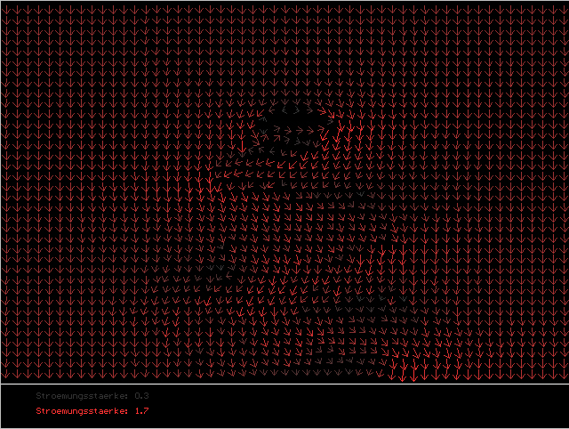
Mode 1:
After the start of the program we are in mode 1 (arow plots). In areas of high pressure the arrows are drawn light red, in areas of very low density the arrows are gray. The scale can be manipulated:
Press:
‚d‘ to increase the high value
‚c‘ to decrease the high value
‚f‘ to increase the low value
‚v‘ to decrease the low value
Also the arrow- sizes can be changed:
Press:
‚g‘ to increase arrow- length
‚b‘ to decrease arrow- length
‚h‘ and ‚n‘ to adjust the size of the arrow- heads
Finally it is also possible to change the number of arrows drawn:
Press:
‚a‘ to increase the number of arrows from left to right
‚y‘ to decrease this number
‚s‘ to increase the number of arrows from top to bottom
‚x‘ to decrease this number.
Arrows are plotted after each change.
Pressing ‚w‘ takes you to mode 2.
Mode 2:
In mode 2 streamlines are drawn.
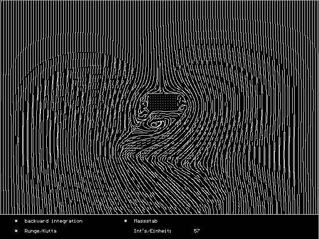
Here you can, for example, choose the kind of integration to be used:
Press:
‚r‘ to toggle between Euler- and Runge/Kutta- integration.
You can also manipulate the density of the streamlines:
Press:
‚a‘ to decrease density
‚y‘ to increase density
Press ‚q‘ to toggle backward integration on and off.
By pressing ‚b‘ you can choose, whether new seed points should be located near the seedpoints of the old streamline or near the ending point of bacwards integration.
It is also possible to change the number of integration steps done within each unit of space.
Press:
‚h‘ to increase that number and
‚n‘ to decrease that number.
The higher the number the smaller the timestep used for integration.
After each change the streamlines are drawn, so changes have an immediate effect.
Press ‚w‘ to get to mode 3
Mode 3:
In this mode evenly based streamlines are drawn. Their construction is based on the algorithm suggested by Bruno Jobard and Wilfrid Lefer.
Changes here have no immediate effect, because drawing takes longer than in modes 1 and 2.
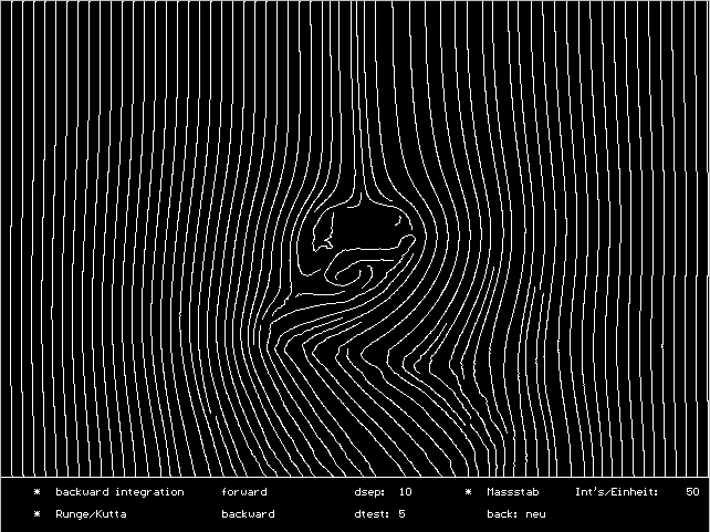
The kind of integration, whether to use backward integration, the parameter for seed point selection and the timestep can be chosen as in mode 2.
Additionally it is possible to choose, which color to use for both forward and backward integration:
Press:
‚f‘ to toggle the color used for forward integration between white and red
‚v‘ to toggle the color used for backward integration between white and red
The parameters dsep and dtest define the density of the streamlines they can be changed as well:
Press:
‚a‘ to increase dsep
‚y‘ to decrease dsep
‚s‘ to increase dtest
‚x‘ to decrease dtest
After choosing the parameters you can press ‚d‘ to draw the streamlines.
Pressing ‚w‘ takes you back to mode 1.