Two dimensional flow visualization
© Alexander Cech - for VISLU 1999/2000
[ Abstract | Input
Data, Downloads | User Interface | Screen
shots ]
Abstract
The program provides visualization of 2-dimensional flow data either as
an arrow plot ("hedgehog") or as streamline diagram.
Input Data
In addition to the program (download here),
you need a data set to visualize.
**********************************************************************

Slice of Direct Numerical Simulation (DNS) of a flow around a block
Use under the condition that the people who generated the data
are properly mentioned:

The data is generated by R.W.C.P. Verstappen &
A.E.P. Veldman of the university of Groningen (the Netherlands)
The technique used to generate the data is described in:
    R.W.C.P. Verstappen & A.E.P. Veldman, 1998: Spectro-consistent
    discretization of Navier-Stokes: a Challenge to RANS and LES,
    Journal of Engineering Mathematics, Vol. 34, pp. 163-179

**********************************************************************
The data set format is described here.
A sample data set (gz-compressed) can be downloaded from here: geometry
(450K) and data
(2.4M) (you need both files).
To unzip the gz-compressed files, you can use WinZip.
User Interface Description
The main window is separated in 3 areas:
Mode Selection Area
Tab "Display"
Here the main properties of the currently loaded data set are displayed.
You can also directly enter the plot coordinates and image scale here.
Image scale: how many pixels to use for 1 data set-unit.
The larger this value is, the larger the plot will be.
X0,X1,Y0,Y1: restrict the plot to a subsection of the
whole data set. (X0,Y0) represents the top left corner, (X1,Y1) the lower
right corner.
Click Auto Scale to calculate the image scale so, that
the plot exactly fits into the display area.
Click Full data set to set the subsection rectangle to
the full data set size.
Click Flip X/Y to mirror the data set along it's second
median. This is useful, if the aspect ratio (= width : height) of the data
set is very different of the aspect ratio of the program window.
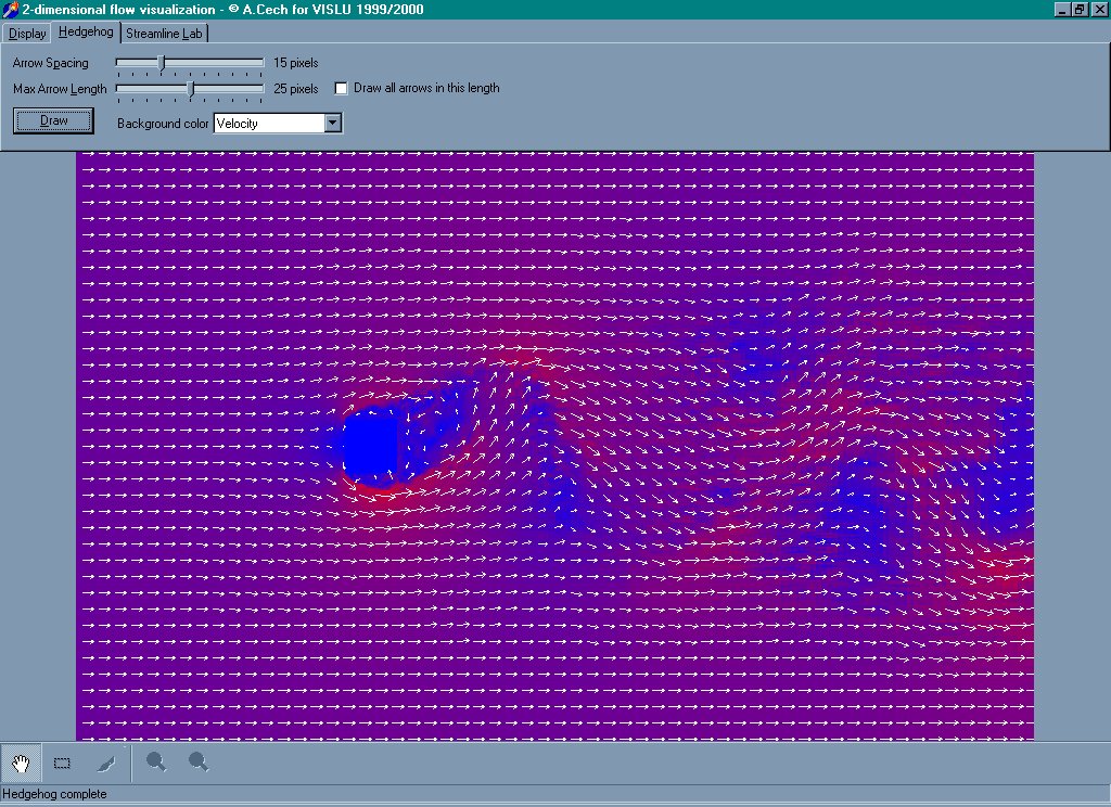
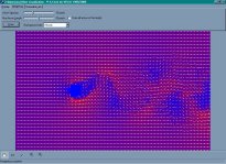
Tab "Hedgehog"
Here you can render an arrow plot ("hedgehog") of the data set.
Specify the spacing between arrow roots and the maximal arrow length
with the sliders.
By checking Draw all arrows in this length, the velocity
component of the data set is ignored and only the flow direction is represented
in the plot.
You can also select a component of the data set to be displayed as
background color. If this option is selected, blue represents the minimal
red the maximal value of the selected data component.
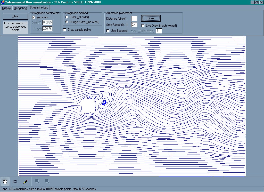
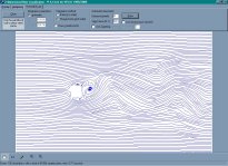
Tab "Streamline Lab"
Here you can calculate streamlines.
A streamline is the path a particle would follow if thrown into the
flow at a specific point.
Use the Paintbrush tool from the toolbox area to place
a particle somewhere in the flow and watch what would happen.
(Note: time is simulated forward and backward, so you don't just see
where the particle would go, but also where it would have come from.)
Click the Clear button to clear the plot area.
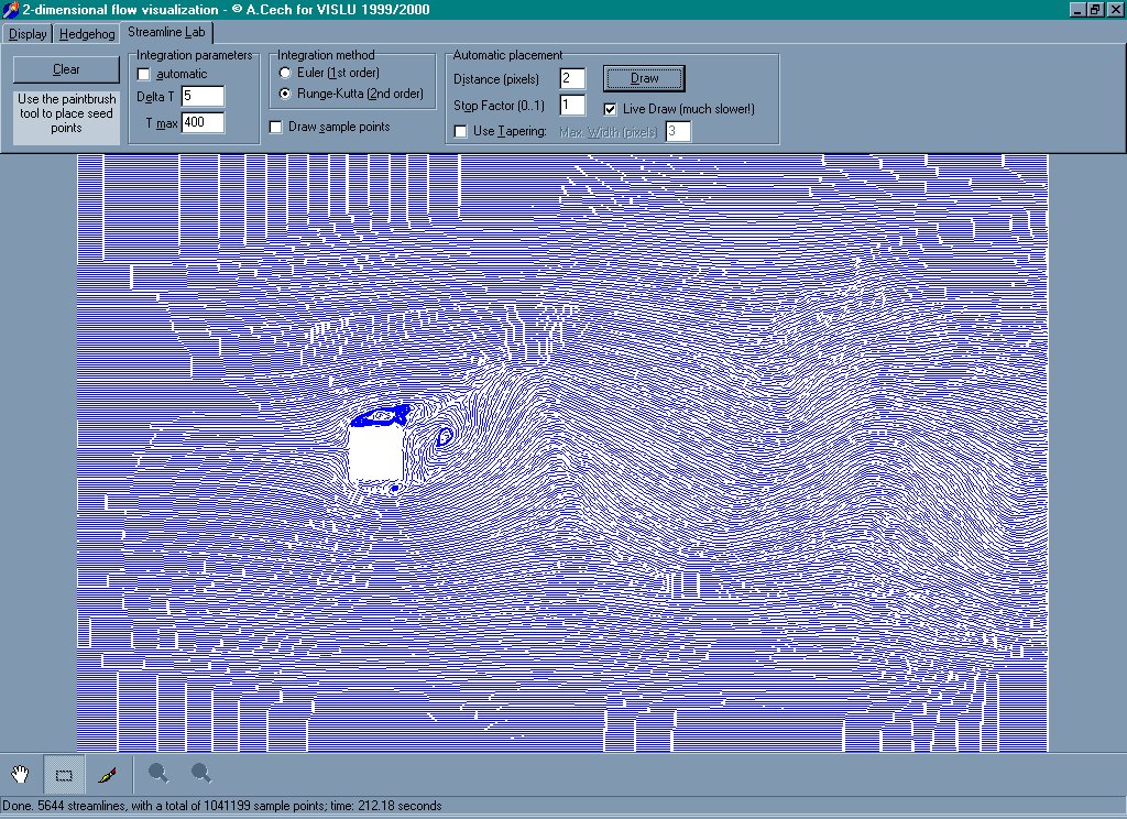
Integration parameters:
Delta T: this is the simulated time step taken
between two successive point on the streamline. The lower this value is,
the more accurate the streamline will be, but the longer it will take to
render.
T Max: if during simulation the streamline does not leave
the plot area in this amount of (simulated) time, drawing is stopped. This
is necessary, since it is perfectly possible for particles to get trapped
flowing around in an endless loop.
Check automatic to let the program choose appropriate
values for Delta T and T Max.
Integration method:
This defines how the particle flow in one time-step is calculated.
Euler (1st order): The flow direction of the current
particle location is simply added to its position.
Runge-Kutta (2nd order): Similarly, the flow direction
of the current location is used to see where the particle would go if the
Eulerian method were used. Now the mean between this vector and the flow
direction vector of the hypothetical particle destination coordinates is
used to calculate the new particle location, giving a more accurate simulation.
If you want to see the actual sample points (= interim particle locations)
calculated, check Draw sample points.
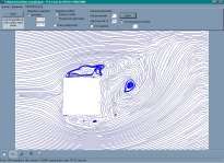
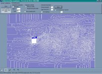
Automatic placement:
In order to cover the whole plot area with streamlines of equal
density an algorithm developed by Bruno Jobard and Wilfrid Lefer is used.
If you are interested, you can find the article here.
Distance (pixels) determines the maximal distance between
two streamlines in pixels.
Stop Factor is a scale factor for the above value. Their
product determines the minimum distance between two stream lines.
(Note: Distance and Stop Factor correspond
to dsep and dtest respectively in Jobard's
and Lefer's article.)
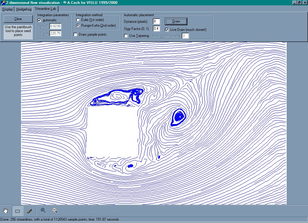
Check Live Draw to see the streamlines being painted
during calculation. This slows things down, but can give you an early impression
of the final image, as well as an approximation of how far the rendering
process is completed.
Check Use Tapering to taper stream line ends. This function
is still under development and does not currently give very nice results.
Click Draw to start the rendering process. If you want
to stop while the plot is not yet completed, just click the same button
again.
Note: When using automatic for the Integration parameters
in conjunction with a high streamline density, rendering time as well as
memory consumption dramatically increases. You can often get equally nice
results in a much shorter amount of time by setting Delta T
to a higher value and decreasing T Max.
Plot Area
This is where the calculated plots are displayed and where you apply the
selected tools from the toolbox.
Toolbox Area
This area consists of 3 tool buttons and 2 zoom buttons.
-
 Drag:
If the Drag tool is selected and the current plot is larger
than the display area, you can click and drag with the mouse to pan the
plot.
Drag:
If the Drag tool is selected and the current plot is larger
than the display area, you can click and drag with the mouse to pan the
plot.
-
 Select:
With the Select tool enabled, click and drag in the display
area, to select a subsection. Hold down the Shift key while dragging
to preserver the aspect ratio.
Select:
With the Select tool enabled, click and drag in the display
area, to select a subsection. Hold down the Shift key while dragging
to preserver the aspect ratio.
-
 Paintbrush: In Streamline Lab mode, select the Paintbrush
tool, and click inside the plot area to render a streamline. You can also
keep the left mouse button pressed while moving the mouse around to generate
a series of streamlines.
Paintbrush: In Streamline Lab mode, select the Paintbrush
tool, and click inside the plot area to render a streamline. You can also
keep the left mouse button pressed while moving the mouse around to generate
a series of streamlines.
-
 Zoom In:
First select a subsection from the plot area (with the Select
tool), then click Zoom In to select and enlarge this area
for plotting. You can achieve the same effect by typing in coordinates
directly in the Display Info tab.
Zoom In:
First select a subsection from the plot area (with the Select
tool), then click Zoom In to select and enlarge this area
for plotting. You can achieve the same effect by typing in coordinates
directly in the Display Info tab.
-
 Zoom Out:
This button doubles the plot subsection rectangle by two in each direction.
Zoom Out:
This button doubles the plot subsection rectangle by two in each direction.
Screen shots
(Click on the thumbnails to see the images in original size)
[ Abstract | Input Data,
Downloads | User Interface | Screen
shots ]
[ Back to top of page ]