| File / Open Dataset |
load a data set into memory |
| File / Load session parameters |
load settings |
| File / Save session parameters |
save all current settings (excluding the data
set) to a file |
| File / Exit |
terminate Data Viewer |
| |
|
| Options / Windowing |
displays the windowing window |
| Options / Transfer Functions |
displays the transfer functions window |
| Options / Live drag |
immediately update display when dragging slice-lines |
| Options / Show drag lines |
display slice drag lines |
| Options / Live Raycast |
display so far rendered image while rendering
is in progress |
| |
|
| Raycast / Edit parameters |
display the raycast parameters window |
| Raycast / .... |
some shortcuts to settings in the raycast parameter
window |
| Raycast / Render |
renders the data set, using data cached from
the previous rendering |
| Raycast / Free and Render |
renders the data set from scratch |
| Raycast / Free memory |
frees data cached from the previous rendering |
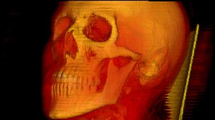
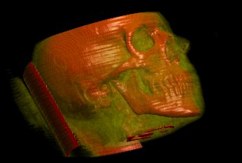
Sample Images
|
View 1
Rotation: X:90° Y:38° Z:0°
Shading: TF
Classification: Simple TF
Phong shading:
20%, 80%, 0%, 0%
Light: 1, -1, 0
Exponent: 200
Trilinear Interpolation |
|
|
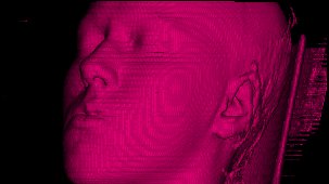
View 2
Rotation: X:90° Y:38° Z:0°
Shading: TF
Classification: Simple TF
Phong shading:
20%, 80%, 0%, 0%
Light: 1, -1, 0
Exponent: 200
Trilinear Interpolation |
|
|
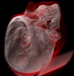
View 3
Rotation: X:0° Y:230° Z:0°
Shading: TF
Classification: Multiple Isov.
Phong shading:
20%, 80%, 0%, 0%
Light: 0, -1, 1
Exponent: 200
Trilinear Interpolation |
|
|
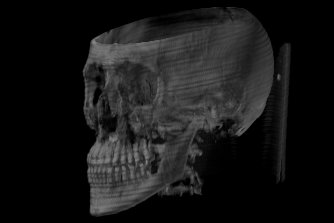
View 4
Rotation: X:103° Y:45° Z:0°
Shading: from Density
Classification: Single Isov.
Phong shading:
20%, 80%, 0%, 0%
Light: 0, -1, 1
Exponent: 200
Trilinear Interpolation |
|
|
View 5
Rotation: X:74° Y:302° Z:0°
Shading: TF
Classification: Simple TF
Phong shading:
10%, 90%, 100%, 5%
Light: -1, -1, 0.5
Exponent: 100
Trilinear Interpolation |
|