The data about artists being player by radio stations is collected using the stations respective "Playing now" webservices.
This data is queried on a regular basis by an AWS lambda function executing the code in src/radio.py.
This simple program calls the webservices and stores their results in a DynamoDB database. Since 3/4 stations use the same format only the fourth requires some normalization (method prepare_886).
The library boto was used for communication with both the webservices and the database. It is preinstalled on AWS Lambda so the program runs as is without dependencies. On a local machine boto might need to be installed.
Note that this will not function without access credentials to said database (using the system's default AWS credentials at ~/.aws/credentials), you can use your own DB by creating a DB called "Radio" in your account as follows:
            "Table": {
                "AttributeDefinitions": [
                    {
                        "AttributeName": "Sender",
                        "AttributeType": "S"
                    },
                    {
                        "AttributeName": "Startzeit",
                        "AttributeType": "N"
                    }
                ],
                "TableName": "Radio",
                "KeySchema": [
                    {
                        "AttributeName": "Sender",
                        "KeyType": "HASH"
                    },
                    {
                        "AttributeName": "Startzeit",
                        "KeyType": "RANGE"
                    }
                ]
            }
The data can be accessed by sender and for a given range of song start times, all other attributes are dynamic. For our purposed the most important one is the "interpreter" 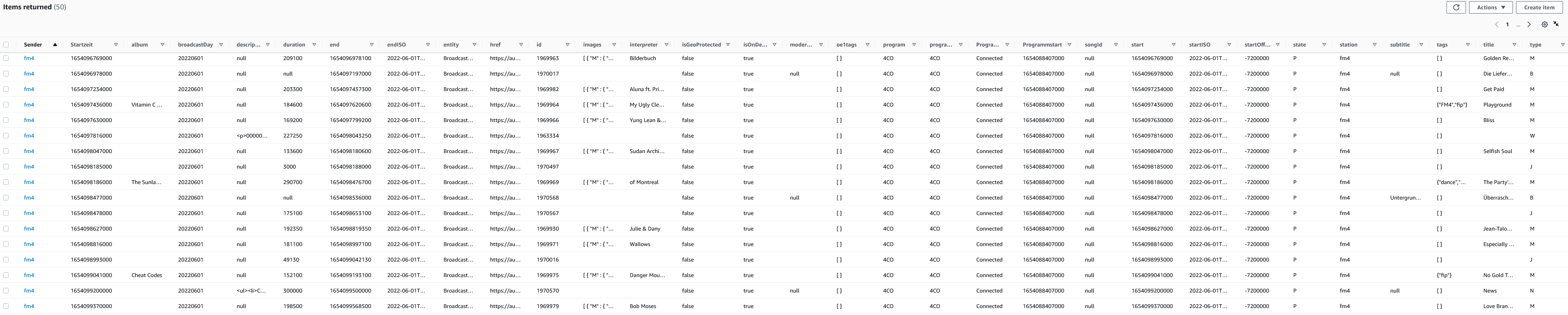
To query and preprocess the data the java program in src/query is used. It connects to the DB using the AWS SDK, using the system's default AWS credentials. Again these need to point to an account with an appropriate DynamoDB.
The program then queries minimal information about the songs for a given month (methods "queryMonth" and "queryRange"), groups them by sender and artist and prints them out in a "json-friendly" format that only needs minimal manual processing before being stored in the appropriate json file along with the program's main html file.
While the query and grouping could be done from the main application it is deliberately implemented as a separate step to avoid repeated queries to the database (especially from the hall of fame) as queries incur charges to the hosting AWS account and the database might be deleted after the course is completed.
The main page consists of two columns that fold into rows if the screen is too narrow.
One contains a set of buttons that can show the following for each of the months with available data:
To compare results we also included representation created by the external library Venn.js.
This diagram is created by the function makeVennJsDiagram that first assures uniqueness within the artists of one station. This data is used to populate the linked table.
Afterwards all possible intersections are calculated and formed in the libraries preferred structure. Finally the library is called to draw the diagram and the data is linked to the table.
While this approach yields quick results it also is not able to display all intersections. E.g. in April there was one artist played in all stations but that intersection is not visible.
The method createDual mostly refers to chapter 5 in the paper.
First the data is prepared in a similar way to chapter 4 but in a more flexible way and with a different data structure. Every unique set of artists for one station immediately becomes a node at rank 1.
Since nodes of rank 2 represent intersections in the data of two stations (and rank 3 for 3 stations etc), they are created just that way. Every rank n > 1 is created by intersecting the nodes at rank n-1 with another rank 1 node they dont already "have". This is done in the method addRank (and it's surrounding loop).
The nodes keep track of what they have been intersected with in the "sources" property to avoid intersecting the same rank 1 node multiple times (A ∩ B ∩ B = A ∩ B) as well as creating the same intersection multiple times just in a different order (A ∩ B = B ∩ A)
Helper functions hasOverlap/getOverlap and allOverlap (checks if all items are the same but possibly in another order) assist with that decision.
Next, the function calculateConsecutiveOnes performs a simplified version of the CO heuristic that determines the number of possibly consecutively connected nodes in an adjacency matrix to help with insertion order later.
The function createGroupFromRank1Nodes then builds groups of nodes that define the basic insertion order. This is done via set extension, the first group is always the first rank 1 node and for every other group one rank 1 node and all other connected nodes are added to the group.
Afterwards we start to actually insert nodes into the rank based dual, starting with a node representing the empty set as root node. As data structure for the dual itself we chose a Map of rank to arrays of nodes.
All nodes also get a property "x" which describes it's position within the rank and an "id" that contains both the rank and x in the form of rank*100+x, thus one rank can hold up to 100 nodes without id overlaps.
Nodes are inserted by group and then by rank. Within the rank they are sorted by the precalculated consecutive ones as well as the number of monotone faces they would produce. Those are calculated in the method countMonotoneFaces.
Because a monotone face must be surrounded by exactly four links, the method detects monotone faces by looking for neighbouring nodes that connect to the same node on the previous and next rank respectively. Also those links must not have any crossings as those would destroy the face.
countMonotoneFaces can process the existing state of the dual and add a node or remove a connection temporarily to test for the change that would cause.
Testing if the connections have crossings is done in the method getCrossings. The input is one link and a crossing is detected if another link begins on one side (based on the node's "x" property) of the link's source and ends on the other side of the link's target.
Note that since the dual only allows connections to an adjacent rank only connections between the same ranks are considered.
Finally all introduced crossings are removed again using the method resolveCrossings. First it checks for every connection if a crossing was introduced using getCrossings as described above. If a crossing is detected we check if removing the connection would cause the graph to become disconnected using the method isConnectedWithoutSingleConnection as well as whether we would destroy a monotone face using countMonotone faces.
If neither is the case the connection is removed.
The test in isConnectedWithoutSingleConnection compares the number of nodes reachable from the root node via tree traversal while ignoring a given connection (implemented in the method traverse) with the complete number of nodes in the dual. If they are equal the graph is connected.
This is repeated until all nodes have been inserted.
Layouting starts with the highest available rank. If that is just one node it is placed in the center and that rank is otherwise skipped.
For every other rank we first assign a concentric circle and determine the total number of connections leading there from the previous rank. Then every node is assigned a portion of the circle proportial to its own number of connections.
This pattern grows outwards until the outermost circle contains the single set nodes at rank 1. The "rank 0" containing the empty set is not placed.