Visualization of dynamical systems

As a dynamical system usually is a very dense representation of a multi-dimensional amount of complex information, the need for visualization is obvious. Many useful techniques are already available. Especially for two- and three-dimensional flow fields many visualization techniques have been developed in the past years [67].

However, the entirety of all kind of dynamical systems is much too diverse to be addressed by a single visualization technique. There is too much difference between, for instance, a discrete and a continuous dynamical system. In general, a proper visualization technique is dependent on the kind of data to be visualized, and the specific goal of investigation. Thus, a separation of techniques according to the specific sub-class of dynamical systems addressed, is necessary.

  

Figure 1.3: Different ways of viewing dynamical systems.

One possible way of classifying visualization techniques for dynamical systems is to look at the data scale they focus on. Stressing the aim of maximizing information transmission through the visual channel, it becomes clear that different visualization techniques are necessary for different scales. Investigating a specific dynamical system locally allows to view many more details simultaneously than analyzing an entire class of dynamical systems. A separation into three levels of data scale is useful for identifying different kinds of visualization techniques (see Fig. 1.3):

Visualizing classes of dynamical systems -

dynamical systems as defined in Eqs. 1.1 are dependent on phase space and parameter space, i.e., $\Omega\!\times\!\Pi\subseteq\mathbf{R}^{n+m}$, in case steady dynamical systems are considered. A visualization of f_p encoding all the dynamics is only possible, if phase space as well as parameter space are of quite low dimensionality, for example, if n+m=2. In Fig. 1.4(a) a visualization of a one-dimensional class of one-dimensional dynamical systems ( $\dot{x} = x^3\!-\!x\!-\!p$) is shown. State variable x is associated with the vertical axis, whereas the only parameter p is mapped to the horizontal axis. Similarities as well as differences between systems with different parameter value p can directly be inferred from the image.

Visualizing one specific dynamical system -

fixing parameters to a specific value, one member out of a class of dynamical systems is depicted. All the available dimensions of the visualization channel can be used to represent information about the single selected system. Techniques belonging to this scale level of visualizing dynamical systems usually map the dynamics in phase space directly into visual properties. Many techniques can be found in this area, especially for system dimensions up to three. There are, however, approaches to the visualization of higher dimensional dynamical systems also [91].

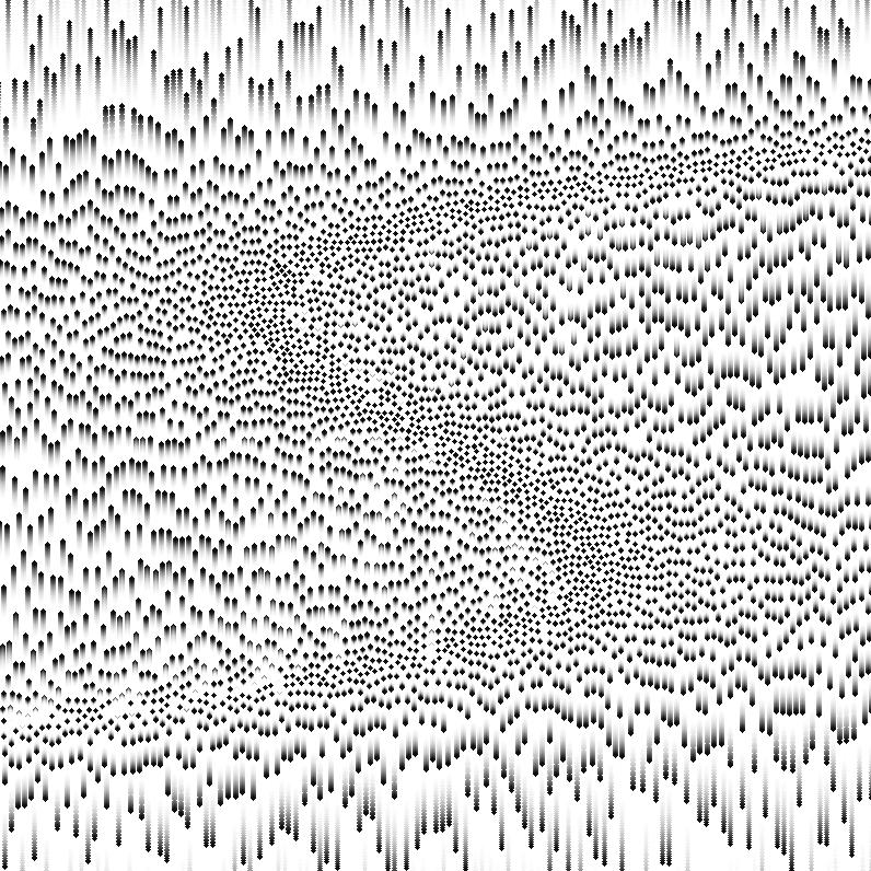
Fig. 1.4(b) shows a two-dimensional visualization of a specific member out of the class of Lotka-Volterra models (cf. Eq. 1.2, $\mathbf{p}=\left(r\ p\ e\ m\right)^\mathrm{T}=\left(1\ 1\ 0.2\ 2\right)^\mathrm{T}$). The dynamics caused by this dynamical system is directly encoded by the used visualization technique.

Visualizing a specific region of interest -

restricting spatial resolution to specific sub-spaces of interest enables the visualization to communicate more details. Data locally available can also be included within the visualization, while neighboring information is omitted.

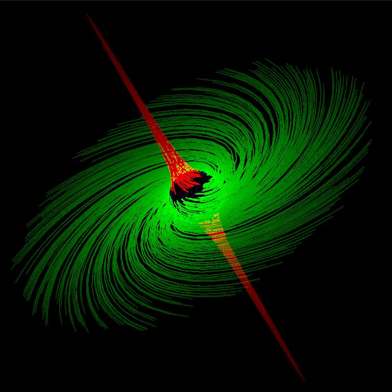
Fig. 1.5(a) shows a visualization of a three-dimensional dynamical system, restricted to a spherical sub-space around the critical point of this system. Although phase space is three-dimensional this local technique avoids visual overloading while still preserving direct visualization of the system dynamics.

  

Figure 1.4: (a) Visualizing a 1D class of 1D dynamical systems - the parameter is varied along the horizontal axis.  (b) Visualizing one specific 2D dynamical system.

  

Figure 1.5: (a) Visualizing a local sub-space of interest [44].  (b) Typical bifurcation diagram.

In general, there are two principal possibilities for designing a visualization technique: direct visualization means to directly map principal flow properties like direction and velocity to a visual representation. All the three classes of visualization mentioned above (more or less) belong to this kind of approach.

The visualization of system abstractions, on the other hand, means to first derive second-level properties of the flow like critical points and separatrices, and then visualize the abstract information. At any scale of the underlying data, analysis can be done first, and visualization used afterwards to convey the results. Characteristic structures like, e.g., critical points (system states where there is no motion at all) or cycles (states of a dynamical systems which reoccur after a certain period of evolution), may be extracted using dynamical system analysis, and mapped to visualization cues afterwards.

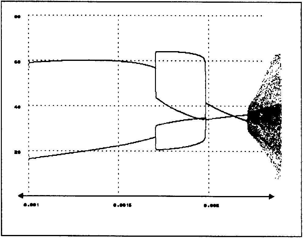
Bifurcation diagrams like the one shown in Fig. 1.5(b) depict (an approximation of) the stable sub-set for each (discrete) dynamical system (1D, vertical axis) in a one-dimensional class (horizontal axis). Bifurcations occur at parameter-value changes, where the stable sub-set changes qualitatively, e.g., at points of a phase doubling or a torus beak-down [77].

  

Figure 1.6: (a) Visualizing an abstraction of a three-dimensional dynamical system [44].  (b) Visualizing the results of local analysis [19].

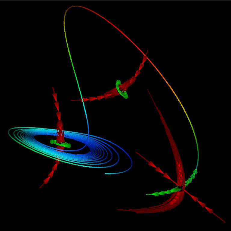
A typical result of visualizing a dynamical system after doing some analysis first, can be seen in Fig. 1.6(a). The critical points are visualized together with the results of an eigenvector and eigenvalue analysis of the system's Jacobian matrix at these points.

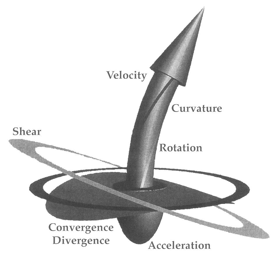
A sample result of visualizing derived data at specific sub-sets of phase space [19] is shown in Fig. 1.6(b). At a specific location in 3D phase space the Jacobian matrix of the dynamical system is analyzed and the derived (local) properties like, direction of flow, velocity, acceleration, rotation, etc., are visualized using a glyph.

An overview of the state of the art in visualizing dynamical systems and related fields is given in Chapter 2. Notes about terms and the local analysis of dynamical systems are given afterwards. Then, four techniques, namely, visualization by the use of stream arrows, visualization based on Poincaré maps, visualizing critical points, and the visualization of characteristic trajectories, are described in Chapters 4, 5, 6, and 7, respectively. A note on the implementation of these visualization methods is appended (Chapt. 8). Finally, a short summary is given, and conclusions are drawn. After the bibliography, a glossary of some important terms related to dynamical systems is given. The thesis concludes with appendices on the notation used and descriptions of the sample dynamical systems used.

mailto:helwig@cg.tuwien.ac.at.