Shading

Despite its lacking physical validity, the Phong illumination model [42] is still widely used in computer graphics. Its popularity is most probably based on its simplicity. Phong's model is a local illumination model, which means only direct reflections are taken into account. While this may not be very realistic, it allows illumination to be computed efficiently. The model consists of an independent ambient, diffuse and specular term. It has the following parameters:

Light vector $L$

The light vector is the normalized vector from a location in space to the light source. In case of a directional light source, this vector is the same for all points in a scene.

View vector $V$

The view vector is the normalized vector from a location in space along a viewing ray to its origin on the image plane. In case of parallel projection, this vector is the same for all points in a scene.

Surface normal $N$

The Phong illumination model was originally designed for the rendering of surfaces. In volume rendering, the surface normal is approximated by the normalized gradient at the resample location.

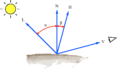
These parameters are illustrated in Figure 3.5. Additionally, the half-way vector $H = \frac{1}{2}(L + V)$ is displayed.

Figure 3.5: Parameters of the Phong illumination model. The light vector $L$ points towards the light source and the view vector $V$ points towards the viewer. $N$ is the surface normal at the point the model is evaluated at. The half-way vector $H$ is the vector half way between $L$ and $V$.

Three constants, $F_{ambient}$, $F_{diffuse}$, and $F_{specular}$, control the contribution of each term to the final light intensity. The shaded color is computed by multiplying the input color (e.g. the color of a sample as obtained through the transfer function) by the sum of the three terms (see Equation 3.7). We assume here that the color of the light source is always white and can therefore disregard its color contribution.

$$c_{out} = c_{in} (I_{ambient} + I_{diffuse} + I_{specular} )$$ (3.7)

The ambient term (Equation 3.8) is constant. Its purpose it to simulate the contribution of indirect reflections, which are otherwise not accounted for by the model.

$$I{}_{ambient} = F_{ambient}$$ (3.8)

The diffuse term (Equation 3.9) is based on Lambert's cosine law which states that the reflection of a perfect rough surface is proportional to the cosine of the angle $\alpha$ between the light vector $L$ and the surface normal $N$.

$$I_{diffuse} = F_{diffuse} \max (L \cdot N,0)$$ (3.9)

The specular term (Equation 3.10)adds an artificial highlight to simulate specular reflections. For computing the specular term, Blinn proposed to use the half-way vector $H$ [1], which is a vector halfway between the light vector and the view vector. The specular lighting intensity is then proportional to the cosine of the angle $\beta$ between the half-way vector $H$ and the surface normal $N$ raised to the power of $n$, where $n$ is called the specular exponent of the surface and represents its shininess. Higher values of $n$ lead to smaller, sharper highlights, whereas lower values result in large and soft highlights.

$$I_{specular} = F_{specular} \max ((H \cdot N)^n ,0)$$ (3.10)

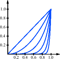
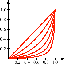
Despite the low complexity of this illumination model, shading still has considerable impact on performance. One way to speed up the evaluation is the use of reflectance maps [52], which contain pre-computed illumination information. However, the use of such data structures requires a considerable amount of additional memory and can lead to cache thrashing. Furthermore, they have to be re-computed every time the illumination properties change. Thus, we choose to evaluate the illumination model on-the-fly. The most time consuming part of the model is the exponentiation used in the specular term. However, since this is a purely empirical model, every function that evokes a similar visual impression can be used instead of the exponentiation. Schlick therefore proposed to use the following approximation [47]:

$$x^n \approx \frac{x}{{n - nx + x}}$$ (3.11)

Figure 3.6: Visual comparison of specular highlights obtained with Phong's and Schlick's approach. (a) Phong. (b) Schlick. The specular exponent is $16$ in both cases.

(a)	(b)

Figure 3.7: Comparison of Phong's and Schlick's approach for specular highlight simulation. (a) Phong: $f(x) = x^n$. (b) Schlick: $f(x) = \frac{x}{{n - nx + x}}.$ $n=1,2,4,8,16,32$.

(a)	(b)

Schlick's approximation is generally much faster to compute and yields to very similar results (see Figure 3.6). Figure 3.7 shows a comparison of the original function and the approximation for different values of $n$.

Our system uses the Phong illumination model with Schlick's approximation for the specular term. One directional light source is supported. This allows us to compute shading at little cost. This setup is well suited for medical applications, where the user generally does not benefit from (and might even be disturbed by) increased photorealism.